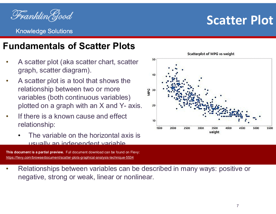
To analyze a scatter plot, you must examine the distribution of points across the Cartesian plane to identify patterns, trends, clusters, and outliers. By plotting two quantitative variables against one another, you can determine if a correlation exists, measure its strength, and identify anomalies that may require further investigation, ultimately turning raw data points into actionable insights.
Understanding the Basics of a Scatter Plot
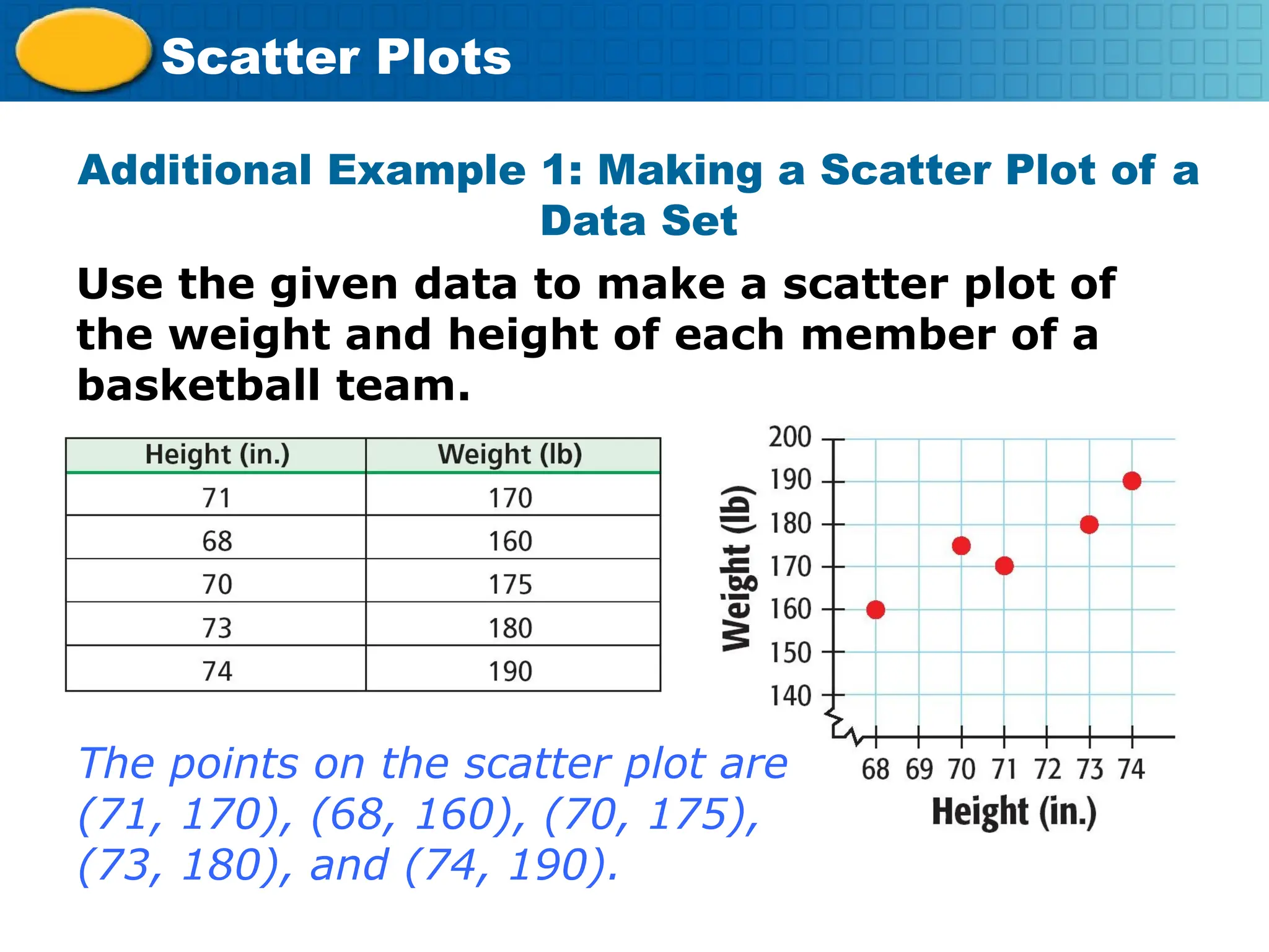
A scatter plot is a fundamental data visualization tool used to observe the relationship between two numerical variables. One variable is plotted on the horizontal axis (the x-axis, or independent variable) and the second variable is plotted on the vertical axis (the y-axis, or dependent variable). Each individual observation in your dataset is represented as a single dot on the graph.
The primary purpose of this visualization is not to show exact individual values, but rather to reveal the overall structure of the data. When you look at a scatter plot, you are essentially performing a visual regression analysis. Before you dive into the data, ensure that your variables are indeed continuous. If you are dealing with categorical data on either axis, a bar chart or a box plot would be a more appropriate choice.
Identifying Correlation and Directionality
The most common task when you analyze a scatter plot is determining if the two variables are related. You do this by looking for the general "shape" the points create.
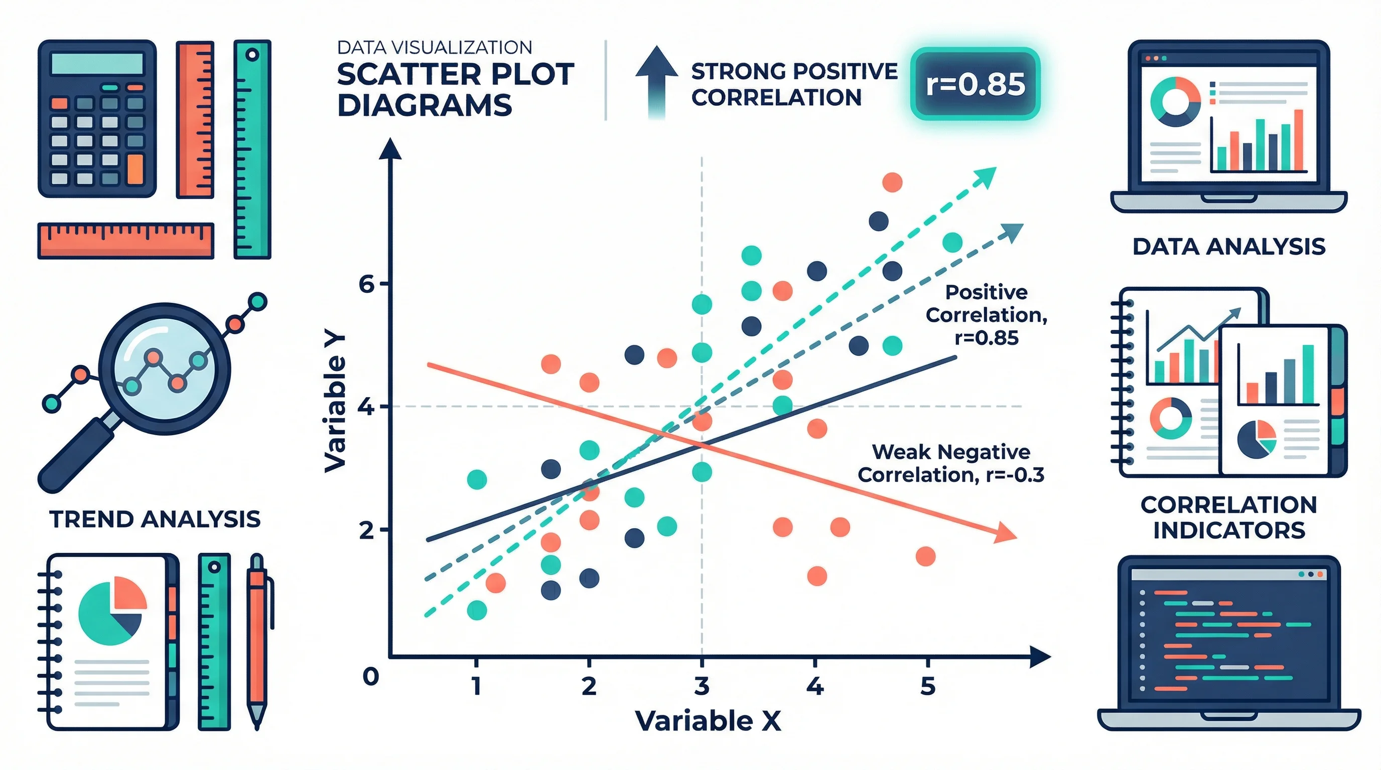
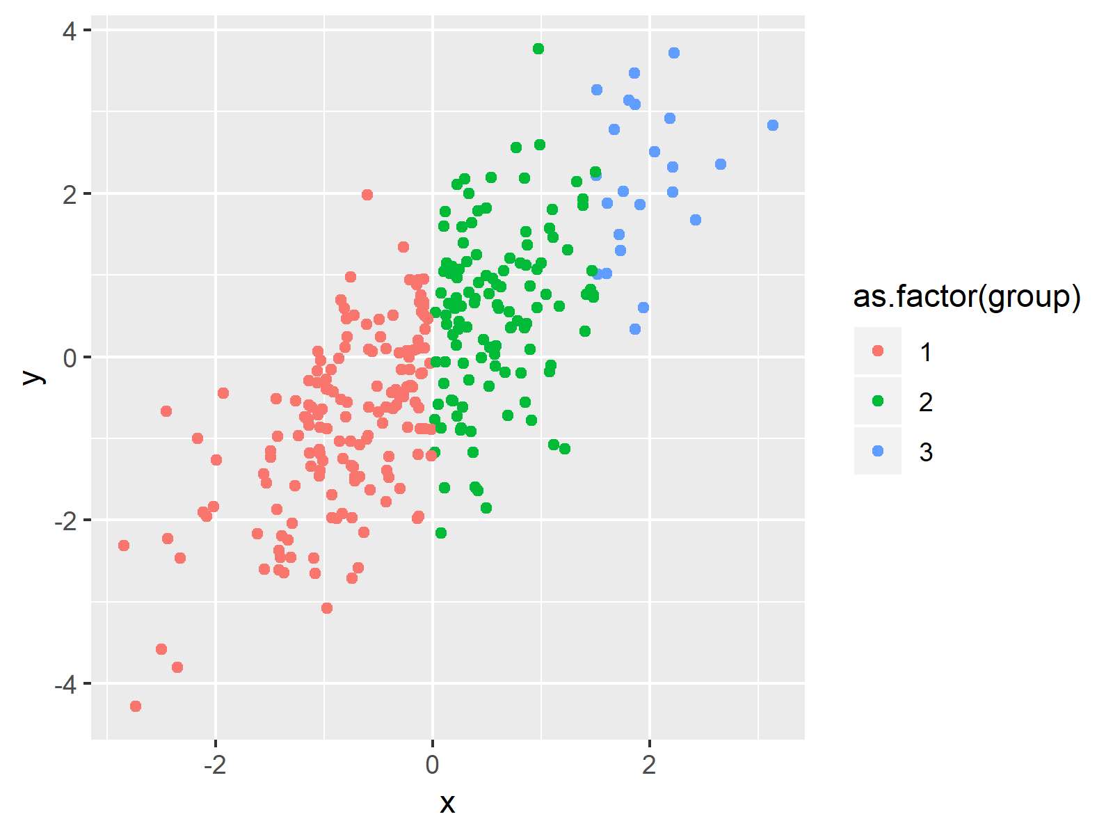
- Positive Correlation: As the value of x increases, the value of y also increases. The points appear to move from the bottom-left toward the top-right of the graph.
- Negative Correlation: As the value of x increases, the value of y decreases. The points follow a downward trend from the top-left to the bottom-right.
- No Correlation: The points are scattered randomly across the plot. There is no discernable line or curve that describes the relationship. In this case, changes in the independent variable do not appear to influence the dependent variable.
Directionality gives you the "what" of the relationship, but it does not tell you everything. A steep upward slope suggests a strong, fast-acting positive relationship, whereas a gentle slope suggests a more subtle connection.
Assessing Strength and Linearity
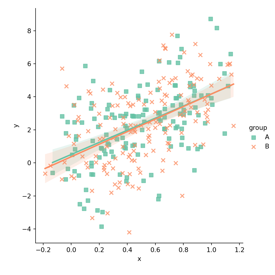
Once you have identified the direction, you must assess the strength of the relationship. This is often described by how closely the points cluster around a theoretical line of best fit (the trendline).
- Strong Relationship: The points are tightly packed together, forming a clear, narrow band. If you were to draw a straight line through the center of the data, nearly all points would fall very close to that line.
- Weak Relationship: The points are spread out widely. While there might be a visible trend, the lack of concentration around a central line suggests that other factors may be influencing the dependent variable.
- Linear vs. Non-Linear: Not all relationships are straight lines. Look for curves. If the points form a "U" shape or an inverted "U," you are looking at a quadratic relationship. If the points start off tight and then spread out significantly, you may be seeing an exponential relationship or an increase in variance (heteroscedasticity).
Detecting Outliers and Clusters
An outlier is a data point that deviates significantly from the overall pattern of the rest of the dataset. When you analyze a scatter plot, outliers are often the most valuable pieces of information because they represent exceptions to the rule. An outlier could indicate a data entry error, a sensor malfunction, or—most importantly—a unique real-world scenario that warrants a deep dive.
Clusters, on the other hand, are groups of points that appear together in a specific region of the graph. Clusters often suggest that your data is composed of sub-groups. For instance, if you are plotting income versus spending, you might see distinct clusters that represent different demographic or socioeconomic segments. By identifying these clusters, you can segment your data and perform a more nuanced analysis that averages would otherwise hide.
Comparison of Scatter Plot Features
| Feature | Visual Indication | Analytical Meaning |
|---|---|---|
| Trendline | Narrow band of points | High correlation between variables |
| Outlier | Isolated point far from the cluster | Anomaly, potential error, or rare event |
| Cluster | Dense, isolated grouping of points | Presence of distinct subsets in data |
| Scatter | Wide, diffuse spread | Weak or non-existent relationship |
| Curvature | Non-linear shape (e.g., U-shape) | Relationship is not proportional |
Step-by-Step Methodology for Analysis
- Define the Variables: Clearly identify what the x and y axes represent. Ensure the units of measurement are appropriate for the analysis.
- Inspect the Axes: Look for the range of data. Are there truncated axes that make a weak relationship look strong? Always be wary of charts that do not start at zero if the context requires it.
- Draw a Mental (or Digital) Trendline: Imagine a straight line that minimizes the distance between itself and all points. Does this line represent the data well?
- Check for Residuals: Consider the distance between each point and your trendline. Are the points consistently far from the line, or are they tightly held?
- Investigate Anomalies: If you spot an outlier, trace it back to the original source. Determine if it is a "dirty" data point or a genuine insight that provides context for your analysis.
- Apply Contextual Knowledge: A scatter plot shows the mathematical relationship, but it cannot confirm causality. Just because two variables correlate does not mean one causes the other. Always cross-reference with domain-specific theories.
Common Pitfalls to Avoid
A frequent error is the assumption that correlation implies causation. If you see a scatter plot showing that ice cream sales and sunscreen sales are both high, it does not mean ice cream causes people to buy sunscreen. Both are likely influenced by a third, hidden variable: summer weather.
Another mistake is failing to account for the scale of the axes. A graph can be manipulated to make a relationship look stronger than it is by zooming in on a very small section of the data range. Always ensure the scale is appropriate to the full range of the dataset. Finally, ignore "data noise"—if your dataset is too small, you may see patterns that are purely coincidental. Always aim for a sufficient sample size to ensure your analysis is statistically representative.
Frequently Asked Questions
Does a scatter plot always show a correlation? No. Many scatter plots show no correlation at all, resulting in a random "cloud" of points. This is still a valid result, as it tells you that the two variables you are comparing do not share a linear relationship.
What should I do if my scatter plot shows a curve? If the relationship is clearly non-linear, a standard linear regression will not be accurate. You may need to use non-linear regression models, such as polynomial, logarithmic, or exponential models, to better represent the data.
How do I handle outliers? Do not immediately delete outliers. First, determine if they are errors (like a typo) or meaningful variations. If they are valid data points, consider if they represent a separate sub-population that should be analyzed independently.
Can I plot more than two variables? A basic scatter plot only handles two. To include a third, you can use "bubble charts" (where the size of the point represents the third variable) or color-code points to represent a categorical third variable.
What if my data is too dense to read? If your plot has thousands of points, it may become an unreadable "inkblot." In this case, use techniques like point transparency (alpha blending), heatmaps, or binning to aggregate the points and reveal the underlying distribution.
Next Steps for Deeper Analysis
Once you have mastered the visual interpretation of a scatter plot, the logical next step is to calculate the Pearson correlation coefficient (r). This statistic provides a numerical value between -1 and +1 that quantifies the strength and direction of the linear relationship you observed. By combining visual inspection with quantitative metrics, you move from simple observation to rigorous data science, allowing you to build predictive models or make evidence-based business decisions. If your analysis reveals a strong trend, consider performing a linear regression to predict future values based on your current data trends.