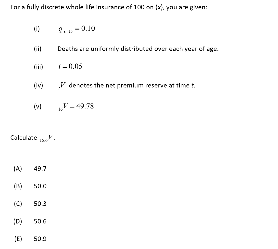
A $150,000 fully discrete whole life insurance policy is a permanent contract where the death benefit remains fixed at $150,000, premiums are paid annually at the beginning of each year, and the death benefit is assumed to be paid out at the exact end of the policy year of death. The standard deviation of life—or more accurately, the standard deviation of the present value of future benefits—is a foundational actuarial metric used to measure the dispersion or risk associated with the timing of the insured's death under mortality assumptions.
Introduction to Fully Discrete Whole Life Insurance and Actuarial Risk
Evaluating life insurance products requires moving beyond simple premium quotes and cash value projections into the realm of actuarial science. A fully discrete whole life insurance policy is a theoretical and practical cornerstone of actuarial mathematics. In this context, "fully discrete" means that premium payments occur at discrete intervals (typically annually) and the death benefit is distributed at the end of the year of death, contrasting with continuous models where payments and transitions happen instantaneously.
For a policy with a face amount of $150,000, the insurer faces a fundamental risk: uncertainty regarding when the insured will die. While mortality tables like the CSO (Commissioners Standard Ordinary) tables provide statistical probabilities of death at various ages, individual outcomes vary significantly. This variance is mathematically captured by calculating the standard deviation of the present value of the future benefit. Understanding this metric allows actuaries, financial analysts, and advanced policyholders to understand how insurers price risk, calculate reserves, and manage solvency for fixed permanent life insurance products.
The Mechanics of Fully Discrete Whole Life Contracts
To comprehend the standard deviation of a $150,000 policy, one must first dissect the structural components of a fully discrete whole life contract. Unlike universal life insurance, which offers flexible premiums and adjustable death benefits, a traditional whole life policy is fixed and guaranteed, provided premiums are maintained.
Premium Payment Structure
In a fully discrete model, the net premium is calculated using the equivalence principle, where the actuarial present value of future premiums equals the actuarial present value of future benefits and expenses. The term "discrete" dictates that premiums are paid at discrete points in time—specifically, at the start of each year ($t = 0, 1, 2, \dots$) that the insured is alive.
Benefit Settlement Assumptions
The death benefit of $150,000 is modeled to be paid at the end of the year in which death occurs. If an individual aged $x$ purchases the policy, and death occurs during the $k$-th year of the policy (between age $x+k-1$ and $x+k$), the benefit is paid at time $k$. This simplification separates discrete models from curtate life-status models, making it mathematically tractable to discount future cash flows using an assumed annual effective interest rate ($i$) or discount factor ($v = \frac{1}{1+i}$).
The Role of Mortality Tables
Actuaries rely on survival models, denoted as $lx$ (number of survivors at age $x$) and $dx$ (number of deaths between age $x$ and $x+1$), derived from population and insured-specific mortality tables. These tables dictate the probability mass function of the random variable representing the future lifetime of the insured.
Defining the Standard Deviation of the Present Value of Benefits
When actuaries speak of the "standard deviation of life" in the context of a life insurance policy, they are mathematically referring to the standard deviation of the present value random variable of the benefits, often denoted as $Z$.
The Present Value Random Variable ($Z$)
Let $Z$ be the present value of the death benefit for a policy issued to an insured aged $x$. If the insured dies in year $K+1$ (where $K$ is the curtate future lifetime, representing the number of complete years lived from age $x$), the present value of the $150,000 benefit is:
$$Z = 150,000 \cdot v^{K+1}$$
Where:
- $v = \frac{1}{1+i}$ is the discount factor.
- $i$ is the assumed annual interest rate.
- $K$ is a discrete random variable taking values $0, 1, 2, \dots$ with respective probabilities determined by the mortality table.
Expected Value Versus Variance
To find the standard deviation, we must first calculate the expected value (mean) of $Z$, denoted as $E[Z]$, and the expected value of the square of $Z$, denoted as $E[Z^2]$.
- Expected Present Value ($E[Z]$): This is the net single premium for a $150,000 term or whole life benefit, calculated by summing the present value of the benefit across all possible years of death, weighted by the probability of dying in each respective year.
- Second Moment ($E[Z^2]$): This is calculated by squaring the discount factor for each year ($v^{2(K+1)}$), multiplying by the benefit squared ($150,000^2$), and weighting by the probability of death in that year.
- Variance ($Var(Z)$): The variance is derived using the standard statistical identity: $$Var(Z) = E[Z^2] - (E[Z])^2$$
- Standard Deviation ($SD(Z)$): The standard deviation is simply the square root of the variance: $$SD(Z) = \sqrt{Var(Z)}$$
| Actuarial Metric | Mathematical Symbol | Description for a $150,000 Policy |
|---|---|---|
| Face Amount | $B$ | Fixed at $150,000 payable at the end of the year of death. |
| Discount Factor | $v^t$ | Present value multiplier based on the technical interest rate $i$. |
| Future Lifetime | $K$ | Curtate future lifetime random variable (completed years of life). |
| Present Value Variable | $Z$ | $B \cdot v^{K+1}$, representing the discounted payout variable. |
| Standard Deviation | $\sigma_Z = \sqrt{Var(Z)}$ | Measures the volatility or dispersion of the policy payout's present value. |
Factors Influencing the Standard Deviation of a $150,000 Policy
The standard deviation of the present value of benefits is not a static number; it fluctuates based on several core demographic, economic, and contract-specific variables.
1. Age at Issue
The age of the insured at the time the $150,000 policy is issued plays a dramatic role in the standard deviation.
- Younger Insureds (e.g., Age 25): The distribution of potential death years is wide, stretching across many decades. Because discounting over 40, 50, or 60 years at compound interest compresses the present value of distant payouts toward zero, the variance of the present value can be surprisingly complex, yet the overall uncertainty of when death occurs creates a substantial spread.
- Older Insureds (e.g., Age 75): The remaining lifetime distribution is compressed into a much narrower window (e.g., 5 to 15 years). Because the time horizon is short, the discounting effect varies less across the remaining probable years of life, which alters the variance profile of the policy.
2. The Assumed Interest Rate ($i$)
Interest rates are a critical parameter in actuarial mathematics. The discount factor $v = \frac{1}{1+i}$ dictates how heavily future cash flows are discounted.
- High Interest Rates: Higher rates shrink the present value of future payouts rapidly. A payout occurring in year 20 is worth drastically less today if the interest rate is 6% versus 3%. This compression reduces the variance ($Var(Z)$), leading to a lower standard deviation.
- Low Interest Rates: Low interest rate environments elevate the present value of distant payouts, increasing the dispersion between early death and late death scenarios, thereby expanding the standard deviation.
3. Mortality Improvement and Table Selection
The underlying mortality table (such as the 2001 or 2008 CSO tables) dictates the shape of the probability distribution. Steeper mortality curves concentrate deaths into a tighter age bracket, whereas flatter curves spread the probability out, directly impacting the calculated variance of $Z$.
Practical Implications for Insurers and Reserves
While standard deviation is a theoretical construct rooted in actuarial mathematics, it has profound real-world consequences for insurance company operations, regulatory compliance, and pricing strategies.
Solvency and Law of Large Numbers
An individual $150,000 fully discrete whole life insurance policy has a high degree of variance when viewed in isolation. An insurer cannot rely on the expected value for a single policyholder because the actual outcome is binary in distribution terms—either the person dies in year one, or they live for decades.
To mitigate this volatility, insurance companies rely on the Law of Large Numbers. By pooling thousands or millions of $150,000 policies, the aggregate standard deviation of the portfolio decreases relative to the portfolio size, allowing the insurer to predict total claims payouts with high statistical confidence.
Statutory Reserves
Insurance regulators require companies to hold statutory reserves to ensure they can meet future obligations. The calculation of net premium reserves (such as the prospective reserve, which is the actuarial present value of future benefits minus the actuarial present value of future net premiums) is directly tied to the expected cash flows that derive from the same mortality and interest assumptions used to find the standard deviation of $Z$.
Common Misconceptions Regarding Whole Life Statistics
When examining technical insurance terms like "standard deviation of life," policyholders and financial students often encounter several persistent misunderstandings.
- Misconception 1: It measures the standard deviation of the insured's lifespan. Many assume that the standard deviation of life refers directly to the statistical variance of human lifespan (e.g., living to age 78 $\pm$ 10 years). While mortality distribution is an input, the actuarial standard deviation specifically measures the present value of the financial benefit ($Z$), incorporating interest rates and discounting, not just raw chronological age.
- Misconception 2: Standard deviation affects annual policy cash value growth. The cash value of a $150,000 whole life policy grows based on the insurer's dividend scale, guaranteed interest rates, and expense charges. It is a contractual accumulation value, not a direct reflection of the policy's mortality variance.
- Misconception 3: All $150,000 policies have identical risk profiles. Two policies with the exact same face value of $150,000 will exhibit entirely different expected present values and standard deviations if issued to individuals of different ages, genders, or health risk classes, due to divergent mortality probabilities.
Step-by-Step Approach to Evaluating Policy Risk Metrics
For analysts or students seeking to evaluate the risk profile of a permanent life insurance contract, a systematic evaluation framework is required.
- Identify Policy Specifications: Confirm the face amount ($150,000), premium frequency (annual fully discrete), and benefit payout timing (end of the year of death).
- Determine Valuation Parameters: Select the appropriate mortality table (e.g., CSO table) and technical annual interest rate mandated by regulatory standards or company pricing models.
- Calculate Expected Present Value ($E[Z]$): Sum the product of each year's discounted benefit and the probability of dying in that specific year.
- Calculate Second Moment ($E[Z^2]$): Square the discount factors, multiply by the squared benefit ($150,000^2$), and weight by the respective death probabilities.
- Compute Variance and Standard Deviation: Apply the variance formula $Var(Z) = E[Z^2] - (E[Z])^2$ and take the square root to determine the standard deviation of the present value of benefits.
Frequently Asked Questions
What does "fully discrete" mean in a whole life insurance contract?
A fully discrete policy is an actuarial model where premium payments occur at discrete intervals (specifically, at the beginning of each year the insured is alive) and the death benefit is assumed to be paid out at the discrete end of the year in which death occurs. This contrasts with continuous models where transactions happen fluidly across every fractional moment of time.
Why is standard deviation important for a $150,000 whole life policy?
Standard deviation measures the dispersion and financial risk associated with the timing of the insured's death. Because insurers must guarantee the $150,000 payout regardless of whether the insured dies next year or fifty years from now, understanding the standard deviation of the present value of benefits is essential for setting adequate reserves and pricing premiums accurately.
How does changing the interest rate impact the standard deviation of benefits?
Higher technical interest rates increase the discounting effect on future payouts, which compresses the range of present values and lowers the standard deviation. Conversely, lower interest rates increase the present value of distant payouts, widening the dispersion of outcomes and increasing the standard deviation.
Does the standard deviation of life affect my personal insurance premiums?
No. The standard deviation is an actuarial risk metric used by insurance companies on an aggregate portfolio level for pricing and reserving. Your individual premium is determined by your age, gender, health classification, and the net single or level annual premium calculations derived from expected mortality values.
Can an individual policyholder calculate their own standard deviation of life?
While individuals can calculate their life expectancy using actuarial tables, calculating the precise standard deviation of the present value of benefits requires complex life table summation, advanced probability weighting for every future year of life, and the specific technical interest rate utilized by the issuing insurance company.
Conclusion and Next Actions
Analyzing a $150,000 fully discrete whole life insurance policy through the lens of the standard deviation of the present value of benefits reveals the sophisticated mathematics underpinning permanent insurance products. By converting mortality probabilities and interest rates into expected values and standard deviations, insurers ensure long-term solvency while providing guaranteed death benefits. For those reviewing existing permanent coverage or studying actuarial science, examining these underlying variance metrics clarifies why fixed-benefit contracts require rigorous underwriting, stable reserve management, and large insurance pools to absorb individual timing risks. To explore specific policy valuations or review your contract's technical disclosures, consult a qualified actuary or review your insurer's statutory annual statement filings.