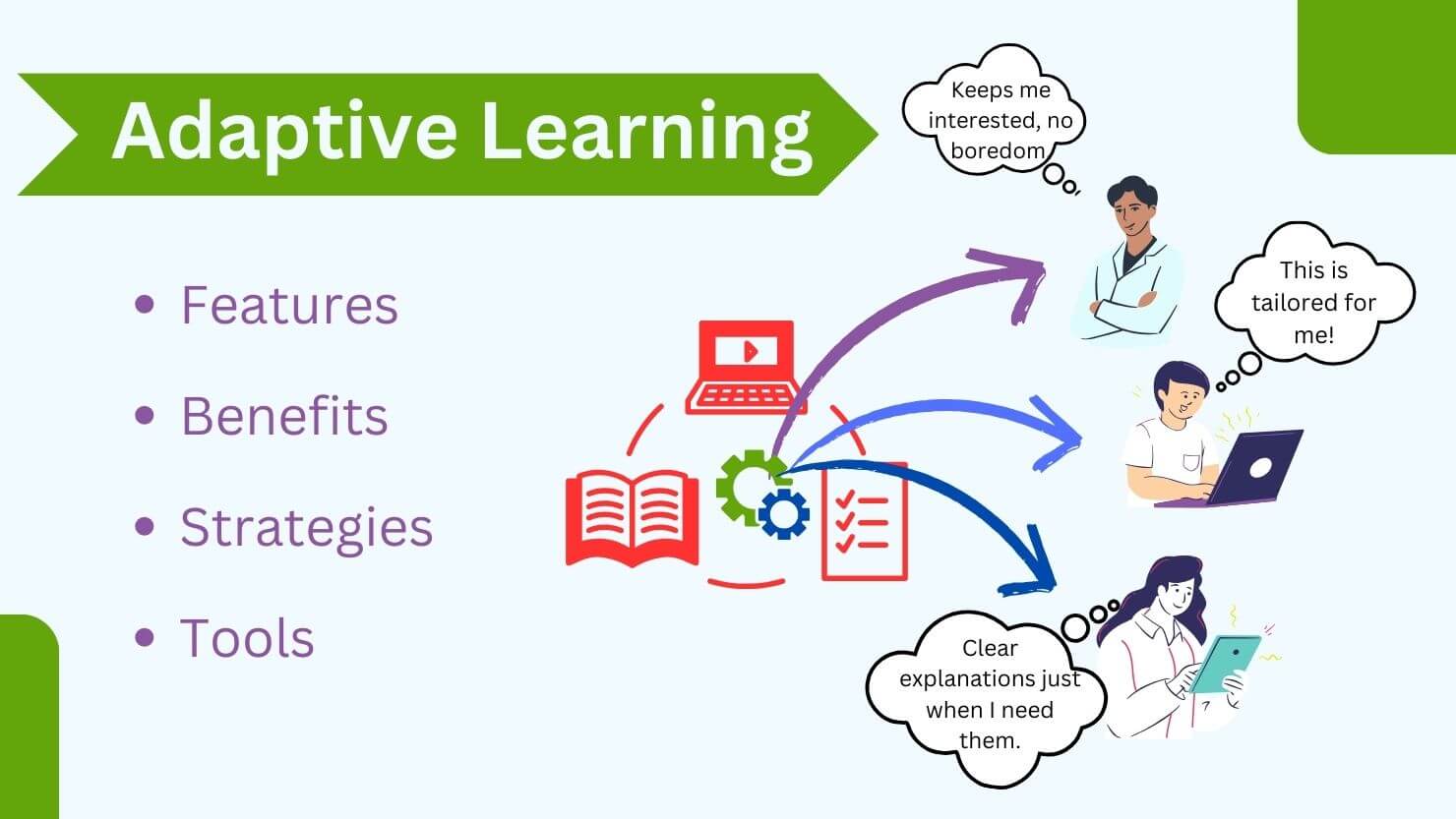
Adaptive learning in machine learning refers to systems that dynamically adjust their internal parameters, architectures, or hyper-parameters during inference or ongoing deployment to handle shifting data distributions and evolving task requirements. Unlike static models trained on fixed datasets, adaptive learning architectures maintain continuous calibration mechanisms to optimize performance without requiring full retraining from scratch.
Foundations of Adaptive Learning in Machine Learning
Traditional machine learning relies on a strict separation between training and inference phases. A model ingests historical training data, updates its weights through backpropagation or optimization solvers, and freezes those parameters for deployment.
While this batch-training paradigm performs well when operating environments remain stationary, real-world data is rarely static. Covariate shift, concept drift, and non-stationary environments frequently degrade the accuracy of static models.
Adaptive learning bridges this gap by embedding mechanisms that allow models to evolve alongside incoming data streams. These mechanisms operate across multiple levels of abstraction, ranging from simple hyper-parameter tuning loops to complex neural architectures with dynamic memory allocation.
The Role of Non-Stationarity in Modern Data
Non-stationarity occurs when the joint probability distribution of inputs and outputs $P(X, Y)$ changes over time. In financial forecasting, consumer behavior alters purchase patterns. In industrial internet of things (IoT) networks, mechanical wear introduces sensor noise and shifts baseline readings.
When a static machine learning model encounters non-stationary data, its predictive performance decays. Adaptive learning algorithms detect this divergence, isolating whether the shift stems from changes in feature distributions ($P(X)$) or conditional relationships ($P(Y|X)$), and trigger targeted updates to preserve model calibration.
Core Paradigms of Adaptation
Implementing adaptability within machine learning requires distinct architectural choices depending on the frequency of data streams and available computational resources. The primary paradigms include online learning, active learning, meta-learning, and continual learning.
Online Learning and Incremental Updates
Online learning algorithms process data sequentially, instance by instance or in small mini-batches, updating model parameters immediately after evaluating each chunk. This approach contrasts with batch learning, which processes the entire dataset simultaneously.
- Stochastic Gradient Descent (SGD): The foundational mechanism for online parameter updates, modifying weights using the gradient computed from a single data point or small sample.
- Recursive Least Squares (RLS): Frequently applied in linear models and adaptive filtering, maintaining an inverse correlation matrix to update coefficients efficiently without recomputing matrix inversions.
- Concept Drift Handlers: Mechanisms such as ADWIN (Adaptive Windowing) or Page-Hinkley tests that monitor error rates to discard outdated data streams dynamically.
Active Learning for Label-Scarce Environments
In many real-world applications, unlabelled data is abundant, but acquiring ground-truth labels is expensive or time-consuming. Active learning allows an adaptive model to query an oracle—such as a human annotator or a high-precision simulation—for labels of the most informative data points.
- Uncertainty Sampling: The model requests labels for instances where its prediction entropy is highest or where class probabilities are near the decision boundary.
- Query-by-Committee: Multiple models vote on unlabelled instances, and data points with the highest disagreement are selected for labeling.
Meta-Learning: Learning to Learn
Meta-learning (L2L) trains models on a distribution of tasks so they can rapidly adapt to new, unseen tasks with minimal data and few gradient steps. Popularized by algorithms like Model-Agnostic Meta-Learning (MAML), meta-learning splits optimization into two loops:
- Outer Loop (Meta-Optimization): Learns an optimal initialization set of parameters across a wide variety of tasks.
- Inner Loop (Task-Specific Adaptation): Fine-tunes the parameters using a small support set from a new task.
Continual Learning and Catastrophic Forgetting
A major challenge in adaptive learning is catastrophic forgetting, where a model updating its weights on a new task overwrites parameters essential for previous tasks. Continual learning addresses this by balancing plasticity (the ability to learn new information) and stability (the preservation of past knowledge).
- Regularization-Based Methods: Penalize changes to important weights, as seen in Elastic Weight Consolidation (EWC).
- Replay-Based Methods: Maintain a small memory buffer of past examples or generate pseudo-samples using generative models to interleave old data with new streams.
Architectural Mechanisms and Comparison
Designing an adaptive machine learning system requires balancing memory consumption, computational overhead, and adaptation speed. The following table compares the primary adaptation paradigms.
| Paradigm | Primary Mechanism | Data Requirement | Main Advantage | Primary Limitation |
|---|---|---|---|---|
| Online Learning | Sequential parameter updates (SGD, RLS) | Continuous streaming data | Low memory footprint; instant updates | Vulnerable to noisy data and catastrophic forgetting |
| Active Learning | Selective querying of informative instances | Unlabelled data + sparse oracle access | Minimizes labeling costs | Requires query latency and oracle availability |
| Meta-Learning | Bilevel optimization (e.g., MAML) | Distribution of related tasks | Fast adaptation to new tasks with few shots | Computationally expensive outer-loop training |
| Continual Learning | Regularization or memory buffers | Sequential task or stream data | Retains past knowledge while learning new tasks | Increased model complexity and memory overhead |
Practical Implementation Steps for Adaptive Systems
Building an adaptive machine learning pipeline involves structured engineering practices to ensure stability, prevent concept drift degradation, and maintain auditability.
1. Establishing Baseline Performance
Before introducing adaptation mechanisms, train a robust static model on historical data. Evaluate its baseline performance using metrics tailored to the problem domain (e.g., Mean Absolute Error for regression, F1-score for imbalanced classification). This baseline serves as a benchmark to quantify the value added by dynamic adaptation.
2. Implementing Drift Detection
Deploy monitoring layers that run parallel to the inference pipeline. Statistical tests—such as Kolmogorov-Smirnov tests for feature distributions or tracking rolling error rates—signal when the divergence between training and inference data exceeds predefined thresholds.
3. Configuring the Adaptation Loop
Select the appropriate adaptation frequency based on operational constraints:
- Real-Time Adaptation: Suitable for high-frequency trading or streaming sensor data where model drift occurs rapidly.
- Scheduled Batch Adaptation: Suitable for weekly or monthly retraining cycles where drift is gradual.
- Triggered Adaptation: Initiated automatically only when drift detectors breach statistical control limits.
4. Guardrails and Validation
Unchecked automated updates can lead to feedback loops or model collapse if poisoned data enters the stream. Implement validation gates that test newly updated weights against a holdout validation set before promoting them to production.
Operational Challenges and Limitations
While adaptive learning offers significant advantages in dynamic environments, practitioners must navigate several inherent risks:
- Catastrophic Forgetting: As discussed, unconstrained adaptation often erases generalized knowledge acquired during initial training phases.
- Data Poisoning Vulnerabilities: In online learning systems that update automatically from user interactions, malicious actors can feed crafted inputs to bias the model over time.
- Computational Overhead: Constantly computing gradients or maintaining memory buffers increases inference latency and infrastructure costs.
- Hyper-Parameter Sensitivity: Adaptive loops introduce meta-parameters—such as learning rates for online updates or drift detection sensitivity thresholds—that require careful tuning to prevent oscillation.
Frequently Asked Questions
What is the difference between online learning and adaptive learning?
Online learning is a specific subset of adaptive learning where models update sequentially as individual data points arrive. Adaptive learning is a broader term that encompasses online learning, meta-learning, active learning, and any architecture designed to adjust to changing operational environments.
How do adaptive machine learning systems prevent catastrophic forgetting?
Systems prevent catastrophic forgetting by utilizing regularization techniques that penalize modifications to critical weights, storing representative historical samples in a replay buffer, or employing modular architectures that allocate dedicated parameter subsets for new tasks.
When should an organization choose meta-learning over standard fine-tuning?
Meta-learning is ideal when an organization frequently encounters distinct but related tasks with very little data available per task (few-shot scenarios). Standard fine-tuning is sufficient when dealing with a single continuous data stream or when abundant target-domain data is available for retraining.
How is concept drift detected in production environments?
Concept drift is detected by monitoring statistical properties of incoming data features versus training distributions using tests like Population Stability Index (PSI), Wasserstein distance, or by tracking rolling performance metrics of the model's predictions over sliding time windows.
Conclusion and Next Actions
Adaptive learning in machine learning provides the necessary architectural foundation for models operating in dynamic, non-stationary environments. By moving beyond static batch training and incorporating online updates, active querying, or meta-learning paradigms, systems can maintain high predictive performance despite shifting data distributions. To begin implementing these concepts, audit your current production models for performance decay, establish statistical drift monitoring on incoming inference streams, and pilot incremental update loops on low-risk auxiliary pipelines.