The 10-Step Guide to Excel SUMIF with 2 Conditions

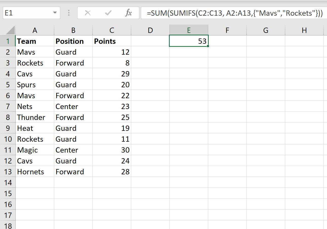
Mastering conditional summation in Microsoft Excel with multiple criteria transforms how you analyze complex datasets. When you need to sum values based on two distinct conditions—such as total sales for a specific region within a specific month—the standard SUMIF function is no longer sufficient on its own because it only accepts a single criteria range. Instead, modern spreadsheet workflows rely on the more versatile SUMIFS function, or legacy multi-criteria workarounds when working in older software versions. This comprehensive 10-step guide covers everything from preparing your data layout to writing, verifying, and troubleshooting multi-condition formulas to ensure absolute accuracy in your financial and operational reports.

Understanding Conditional Summation: SUMIF vs. SUMIFS

Before diving into the multi-step building process, it is vital to understand the structural difference between single-condition and multi-condition aggregation in Excel. The traditional SUMIF function syntax is =SUMIF(range, criteria, [sum_range]). It evaluates a single range against a single criterion and sums the corresponding values in the sum range.

When your data demands two or more conditions—for instance, finding the total revenue generated by "Product A" in the "North" region—you must transition to the SUMIFS function. The syntax for SUMIFS shifts the placement of the sum range to the very beginning: =SUMIFS(sum_range, criteria_range1, criteria1, criteria_range2, criteria2). This syntax allows Excel to evaluate multiple criteria ranges simultaneously, filtering rows that meet every single requirement before adding the numerical values.

Step 1: Structure and Format Your Source Data Correctly

The reliability of any Excel formula depends entirely on the cleanliness of the underlying dataset. Before writing a multi-condition formula, inspect your worksheet layout to ensure it adheres to standard tabular data principles.

1. Uniform Columns and Rows: Ensure your data is organized in a strict tabular format where each column represents a distinct category (e.g., Date, Region, Product, Sales) and each row represents a single, independent record.
2. Eliminate Blank Rows and Columns: Remove completely empty rows or columns inside your data table, as these can disrupt dynamic ranges and cause unexpected formula behavior.
3. Consistent Data Types: Verify that numeric values are stored as actual numbers rather than text strings, and dates are formatted uniformly. Text discrepancies, such as trailing spaces or inconsistent capitalization (e.g., "North" vs. "north "), will cause your conditional criteria to fail silently.

Step 2: Define Your Two Specific Conditions and Target Range

Clarity regarding your analytical objective prevents errors during formula construction. Take a moment to clearly define the exact parameters you want to evaluate.

1. Identify the Sum Range: Determine which numerical column holds the values you want to aggregate (e.g., a column titled Revenue or Quantity).
2. Determine Condition One: Establish your first filter criterion and its corresponding column range (e.g., Region must equal "East").
3. Determine Condition Two: Establish your second filter criterion and its corresponding column range (e.g., Product Category must equal "Software").

Step 3: Set Up a Dedicated Calculation Area

Placing your formulas directly inside your raw data table can lead to accidental overwrites and reference errors when sorting or filtering.

1. Create a separate summary tab or an isolated section on your current worksheet.
2. Clearly label your criteria cells so anyone reviewing the workbook understands what the outputs represent. For example, place "Region" in cell E1 and type "East" in cell F1, and place "Product" in cell E2 and type "Software" in cell F2.
3. Reserve your output cells for the final SUMIFS formula calculations.

Step 4: Write the Basic SUMIFS Function Structure

With your data prepared and your criteria defined, you are ready to construct the formula shell. Click on the destination cell where you want the final sum to appear.

1. Type the equals sign to initiate the formula: =SUMIFS(.
2. Immediately select or type your sum range (the numerical data you want to add up, such as D2:D500).
3. Type a comma to separate the arguments. Your formula should currently look similar to =SUMIFS(D2:D500, .

Step 5: Add the First Criteria Range and Criterion

Next, you will instruct Excel where to look for your first condition and what specific value it must match.

1. Select or type the first criteria range (e.g., the column containing region names, such as A2:A500).
2. Type a comma.
3. Reference the cell containing your first criterion (e.g., F1) or enclose the text criterion in double quotation marks (e.g., "East").
4. Your formula now resembles =SUMIFS(D2:D500, A2:A500, F1, .

Step 6: Add the Second Criteria Range and Criterion

Now, append the second set of parameters to complete the multi-condition evaluation logic.

1. Select or type the second criteria range (e.g., the column containing product names, such as B2:B500).
2. Type a comma.
3. Reference the cell containing your second criterion (e.g., F2) or type the text in quotes (e.g., "Software").
4. Close the parentheses to complete the function syntax: ).
5. Your final formula structure should look like: =SUMIFS(D2:D500, A2:A500, F1, B2:B500, F2).

Step 7: Execute and Test the Formula

Press Enter on your keyboard to execute the formula. Excel will scan the specified ranges, isolate the rows that satisfy both condition one and condition two simultaneously, and return the aggregated sum.

1. Test the output by changing one of your criteria cells (e.g., change "East" to "West") to verify that the returned sum updates dynamically.
2. If the formula returns zero or an error, check that your criteria spelling matches the raw data exactly.

Step 8: Utilize Operators and Wildcards for Advanced Conditions

Real-world data analysis often requires more than exact text matches. You can enhance your two-condition SUMIFS formula by incorporating logical operators and wildcards.

When combining logical operators with cell references, remember to concatenate the operator in quotation marks with an ampersand (&), such as ">"&F3.

Step 9: Common Mistakes and Troubleshooting Techniques

Even experienced spreadsheet users occasionally encounter errors when writing multi-condition formulas. Review these common pitfalls to resolve issues quickly.

• Mismatched Range Sizes: Every criteria range in a SUMIFS function must have the exact same dimensions and row counts as the sum range (e.g., if your sum range is D2:D500, your criteria ranges cannot be A1:A499). Mismatched ranges will produce a #VALUE! error.
• Text Formatting Traps: Invisible leading or trailing spaces within text cells prevent exact matches. Use the TRIM function in a helper column to clean erratic spacing if your formula returns unexpected zeros.
• Locked Cell References: If you plan to drag or copy your formula across multiple rows or columns, ensure you use absolute references (e.g., $D$2:$D$500) to prevent your ranges from shifting unintentionally.

Step 10: Alternative Methods (SUMPRODUCT and Pivot Tables)

While SUMIFS is the most efficient and readable tool for two conditions, alternative approaches exist depending on your reporting requirements.

1. SUMPRODUCT Function: For complex criteria involving boolean logic arrays or calculations performed directly within the criteria, =SUMPRODUCT((A2:A500="East")*(B2:B500="Software")*(D2:D500)) offers a powerful legacy alternative that functions across older Excel versions without crashing.
2. Pivot Tables: If you need to evaluate two conditions across an entire dataset simultaneously without writing long formulas, insert a Pivot Table. Drag your two condition fields into the Rows or Filters area and your numerical field into the Values area to instantly generate a complete multi-conditional summary matrix.

Frequently Asked Questions

Can SUMIFS handle more than two conditions?

Yes. Although this guide focuses on two conditions, the SUMIFS function can accommodate up to 127 criteria range and criteria pairs in modern versions of Excel. Simply continue appending additional range and criteria pairs separated by commas.

Why is my SUMIFS formula returning zero when I know data exists?

A zero result usually indicates that no single row in your dataset satisfies all conditions simultaneously. Check for spelling discrepancies, hidden trailing spaces in text fields, or strict date formatting conflicts where time stamps interfere with calendar day matching.

Can I use OR logic instead of AND logic within SUMIFS?

Standard SUMIFS evaluates conditions using strict AND logic (Condition A and Condition B must both be true). To perform an OR summation across two conditions, you can add two separate SUMIFS formulas together within the same cell, such as =SUMIFS(sum, range, "East") + SUMIFS(sum, range, "West").

How do I sum values based on blank or non-blank cells?

To sum rows where a secondary condition cell is blank, use quotation marks with nothing inside them ("") as your criterion. To sum rows where a cell is not blank, use the inequality operator combined with empty quotes ("<>").

What should I do if my formula returns a #VALUE! error?

A #VALUE! error almost always occurs when the dimensions of your sum range and your criteria ranges do not match precisely. Verify that every range referenced in your formula spans the exact same number of rows and columns.

Conclusion and Next Actions

Mastering the SUMIFS function for two or more conditions significantly boosts your data processing efficiency, replacing cumbersome manual filtering with dynamic, automated calculations. Begin by ensuring your source data is uniformly formatted, structure your formula with careful attention to range alignment, and leverage wildcards or operators for advanced matching. To continue refining your spreadsheet skills, practice building dynamic dashboards that link these multi-condition formulas directly to interactive drop-down menus.