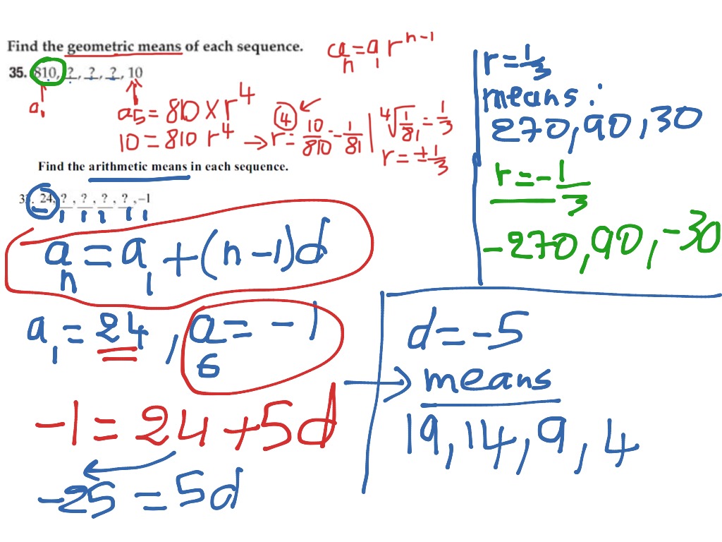
The Arithmetic Mean-Geometric Mean (AM-GM) inequality is a fundamental principle of mathematics stating that the arithmetic mean of a set of non-negative real numbers is always greater than or equal to their geometric mean. This relationship holds for any collection of positive values, with equality occurring only when all numbers in the set are identical.
The AM-GM inequality serves as a cornerstone in various mathematical disciplines, including algebra, calculus, and optimization. By providing a bridge between addition and multiplication, it allows mathematicians and scientists to establish bounds for functions and solve complex optimization problems without always relying on derivative-based calculus. In the current academic landscape of 2026, it remains one of the most frequently utilized tools in competitive mathematics and theoretical physics.
Defining the AM-GM Inequality
To understand the inequality, we must first define the two types of means it compares. For a set of $n$ non-negative real numbers $x_1, x_2, \dots, x_n$:
- Arithmetic Mean (AM): This is the standard "average" most people are familiar with. It is calculated by summing all the numbers and dividing by the total count $n$. $$\text{AM} = \frac{x_1 + x_2 + \dots + x_n}{n}$$
- Geometric Mean (GM): This mean represents the central tendency of a set of numbers by using the product of their values. It is calculated by multiplying all the numbers together and taking the $n$-th root. $$\text{GM} = \sqrt[n]{x_1 \cdot x_2 \cdot \dots \cdot x_n}$$
The AM-GM Inequality states that: $$\frac{x_1 + x_2 + \dots + x_n}{n} \geq \sqrt[n]{x_1 \cdot x_2 \cdot \dots \cdot x_n}$$
The Condition of Equality
A critical aspect of this inequality is the condition under which the two means are exactly equal. The arithmetic mean equals the geometric mean if and only if all the numbers in the set are equal ($x_1 = x_2 = \dots = x_n$). If there is even the slightest variation between any two numbers in the set, the arithmetic mean will strictly exceed the geometric mean.
The Mathematical Proofs of AM-GM
The AM-GM inequality can be proven through several different methods, each offering unique insights into why the relationship holds. Here, we explore the three most significant proofs: the basic algebraic case for $n=2$, Cauchy's induction method, and the proof via Jensen's Inequality.
1. The Proof for $n=2$ (The Foundation)
The simplest case involves only two numbers, $a$ and $b$. This proof relies on the fact that the square of any real number is non-negative.
- Start with the assumption that $(\sqrt{a} - \sqrt{b})^2 \geq 0$.
- Expand the square: $a - 2\sqrt{ab} + b \geq 0$.
- Rearrange the terms: $a + b \geq 2\sqrt{ab}$.
- Divide both sides by 2: $\frac{a+b}{2} \geq \sqrt{ab}$.
This demonstrates the inequality for two variables. It also clearly shows that equality holds only when $\sqrt{a} - \sqrt{b} = 0$, which implies $a = b$.
2. Cauchy’s Backward Induction
Augustin-Louis Cauchy provided a famous proof that uses a unique form of induction. Instead of the standard $n$ to $n+1$ progression, he proved it for powers of 2 ($n=2, 4, 8, \dots$) and then "filled in the gaps" by working backward.
- Step 1 (Forward): We already know it works for $n=2$. By applying the $n=2$ case to pairs of numbers, it is easy to show it works for $n=4$, then $n=8$, and eventually any $n = 2^k$.
- Step 2 (Backward): If the inequality holds for $n$, Cauchy showed it must also hold for $n-1$. This is achieved by setting the $n$-th variable ($x_n$) equal to the arithmetic mean of the first $n-1$ variables.
- By proving it for all powers of 2 and showing that a valid proof for $n$ implies a valid proof for $n-1$, Cauchy covered all possible natural numbers.
3. Proof via Jensen’s Inequality (Convexity)
Jensen’s Inequality relates to the properties of convex and concave functions. This is perhaps the most elegant proof for those familiar with calculus.
- Consider the natural logarithm function, $f(x) = \ln(x)$.
- The second derivative of $\ln(x)$ is $-1/x^2$, which is always negative for $x > 0$. This means the log function is concave.
- Jensen's Inequality for concave functions states that the function of the average is greater than or equal to the average of the function: $$\ln\left(\frac{x_1 + \dots + x_n}{n}\right) \geq \frac{\ln(x_1) + \dots + \ln(x_n)}{n}$$
- Using log properties, the right side becomes $\frac{1}{n} \ln(x_1 \dots x_n)$, which is $\ln(\sqrt[n]{x_1 \dots x_n})$.
- Since the log function is strictly increasing, we can remove the logarithms from both sides: $$\frac{x_1 + \dots + x_n}{n} \geq \sqrt[n]{x_1 \dots x_n}$$
Primary Uses and Applications
The AM-GM inequality is far more than a theoretical curiosity; it is a practical tool used to solve real-world problems in geometry, economics, and engineering.
1. Optimization and Minimum/Maximum Values
One of the most common uses of AM-GM is finding the extreme values of a function without using derivatives.
Example: Find the minimum value of $f(x) = x + \frac{9}{x}$ for $x > 0$. Using AM-GM on the two terms $x$ and $9/x$: $$\frac{x + \frac{9}{x}}{2} \geq \sqrt{x \cdot \frac{9}{x}}$$ $$\frac{x + \frac{9}{x}}{2} \geq \sqrt{9}$$ $$x + \frac{9}{x} \geq 2 \cdot 3 = 6$$ The minimum value is 6, and it occurs when $x = 9/x$, which means $x^2 = 9$ or $x=3$.
2. Geometric Relationships
AM-GM explains many fundamental geometric truths. For instance, among all rectangles with a fixed perimeter, the square has the maximum area.
- Let the sides be $L$ and $W$. Perimeter $P = 2(L+W)$, so $L+W = P/2$.
- Area $A = L \cdot W$.
- By AM-GM: $\frac{L+W}{2} \geq \sqrt{LW}$.
- Substituting the perimeter: $\frac{P}{4} \geq \sqrt{A}$.
- Squaring both sides: $A \leq \frac{P^2}{16}$. The maximum area $A$ is reached only when $L=W$, which is a square.
3. Proving Other Inequalities
The AM-GM inequality is often the first step in proving more complex relationships like the Cauchy-Schwarz inequality or the Bernoulli inequality. It acts as a "building block" in mathematical analysis. In physics, it is used to determine lower bounds for energy states or to bound the rates of thermodynamic processes.
Comparison of Different Means
The AM-GM inequality is actually part of a larger chain known as the Pythagorean Means or the Generalized Mean Inequality. Understanding where AM and GM sit in this hierarchy provides a better context for their use.
| Mean Type | Formula | Sensitivity to Outliers | Common Use Case |
|---|---|---|---|
| Harmonic (HM) | $n / \sum (1/x_i)$ | High (sensitive to small values) | Average speeds, resistance in circuits |
| Geometric (GM) | $\sqrt[n]{\prod x_i}$ | Moderate | Growth rates, investment returns |
| Arithmetic (AM) | $(\sum x_i) / n$ | Moderate | Standard statistical averaging |
| Root Mean Square (RMS) | $\sqrt{(\sum x_i^2) / n}$ | High (sensitive to large values) | Physical magnitudes, electrical voltage |
The relationship between these is: HM ≤ GM ≤ AM ≤ RMS.
Weighted AM-GM Inequality
In some scenarios, not all numbers in a set are equally important. This leads to the Weighted AM-GM Inequality. If we have weights $w_1, w_2, \dots, w_n$ such that their sum is 1, the inequality is expressed as: $$w_1 x_1 + w_2 x_2 + \dots + w_n x_n \geq x_1^{w_1} \cdot x_2^{w_2} \cdot \dots \cdot x_n^{w_n}$$ This version is widely used in economics for calculating price indices and in information theory to calculate entropy bounds.
Common Mistakes to Avoid
While the AM-GM inequality is straightforward, there are several pitfalls that students and professionals often encounter:
- Ignoring the Non-Negativity Constraint: The AM-GM inequality only applies to non-negative real numbers. If the set contains negative numbers, the geometric mean may become an imaginary number or the inequality may simply fail to hold.
- Assuming Equality Too Often: Remember that AM only equals GM if all elements are identical. If you are solving an optimization problem and the variables cannot be equal due to other constraints, the minimum or maximum bound provided by AM-GM might not be achievable.
- Misapplying to Sums of Products: AM-GM is most effective when the product of the terms simplifies to a constant. If the product of the terms still contains variables, AM-GM might not directly lead to a solution for a minimum or maximum.
Frequently Asked Questions
Can the AM-GM inequality be used for zero values?
Yes, the AM-GM inequality remains valid if one or more of the numbers are zero. If any $x_i = 0$, the product becomes zero, making the geometric mean zero. Since the arithmetic mean of non-negative numbers is always $\geq 0$, the inequality $\text{AM} \geq 0$ still holds.
Why is the geometric mean often used in finance instead of the arithmetic mean?
The geometric mean is superior for calculating average investment returns over multiple periods. This is because investment growth is multiplicative, not additive. For example, a 50% gain followed by a 50% loss results in a total loss of 25% (0.75 of original), which the geometric mean reflects accurately, whereas the arithmetic mean would misleadingly suggest a 0% average change.
Does the AM-GM inequality work for complex numbers?
No, the standard AM-GM inequality does not apply to complex numbers because the concept of "greater than" or "less than" (ordering) is not defined for complex numbers in the same way it is for real numbers. Additionally, taking $n$-th roots of complex numbers yields multiple values, complicating the definition of a geometric mean.
What is the history of the AM-GM inequality?
The concept of these means dates back to ancient Greek mathematicians, including Euclid and Pythagoras. However, the formal generalized proof for $n$ variables was most notably advanced by Augustin-Louis Cauchy in the 19th century. His "backward induction" remains a staple of mathematical pedagogy.
How does AM-GM relate to the RMS-AM inequality?
The Root Mean Square (RMS) is always greater than or equal to the Arithmetic Mean. When combined with AM-GM, it forms a chain: $\text{RMS} \geq \text{AM} \geq \text{GM}$. This is useful in statistics to show that the standard deviation (related to RMS) affects the relationship between different types of averages.
Practical Recommendation
When faced with an optimization problem where you need to find the maximum product given a constant sum (or a minimum sum given a constant product), always attempt to apply the AM-GM inequality before moving to calculus. It is often faster, less prone to calculation errors, and provides an immediate "target" value where all variables are equal. For those preparing for mathematical competitions or advanced engineering exams in 2026, mastering the different proofs of AM-GM—especially the Jensen’s Inequality approach—will provide a deeper understanding of the interplay between algebraic structures and functional analysis.