An ANOVA table formula set organizes variance decomposition into Sum of Squares ($SS$), Degrees of Freedom ($DF$), Mean Squares ($MS$), and the test statistic ($F$). For a One-Way ANOVA, the primary formulas are $SS_{\text{Total}} = SS_{\text{Between}} + SS_{\text{Within}}$, $DF_{\text{Between}} = k - 1$, $DF_{\text{Within}} = N - k$, $MS = \frac{SS}{DF}$, and $F = \frac{MS_{\text{Between}}}{MS_{\text{Within}}}$.
Understanding the Structure of an ANOVA Table
Analysis of Variance (ANOVA), first introduced by statistician Ronald Fisher, evaluates differences among group means by partitioning total variability in a dataset into distinct components. Rather than running multiple individual $t$-tests—which inflates Type I error rates—ANOVA uses an $F$-test to evaluate whether at least two sample means differ significantly.
The results of an ANOVA computation are presented in a structured ANOVA table. This table summarizes how variability is split between differences across treatment groups and random variation within those groups.
Every ANOVA table features five primary columns regardless of whether the experimental design is a simple single-factor study or a complex multi-factor factorial experiment:
- Source of Variation: Identifies the origin of variability (e.g., Treatments/Between Groups, Error/Within Groups, or Interaction terms).
- Sum of Squares ($SS$): Measures the total squared deviation attributable to each source of variation.
- Degrees of Freedom ($DF$): Represents the number of independent values or quantities that can vary in the analysis.
- Mean Square ($MS$): The sample variance for a given source, computed as $\frac{SS}{DF}$.
- $F$-Statistic ($F$): The test ratio comparing variance explained by a factor against random error variance.
One-Way ANOVA Table Formulas Explained
A One-Way ANOVA tests the effect of a single categorical independent variable (factor) with $k$ levels on a continuous dependent variable across $N$ total observations.
Mathematical Notation Summary
- $k$: Number of groups or factor levels.
- $n_i$: Sample size of group $i$.
- $N$: Total sample size across all groups ($N = \sum_{i=1}^{k} n_i$).
- $X_{ij}$: The $j$-th observation in the $i$-th group.
- $\bar{X}_{i\cdot}$: Mean of group $i$.
- $\bar{X}_{\cdot\cdot}$: Grand mean of all $N$ observations.
- $T_{i\cdot}$: Sum of all values in group $i$.
- $T_{\cdot\cdot}$: Grand total of all observations across all groups.
Definitional vs. Computational Formulas
When performing manual calculations or programming statistical algorithms, standard statistical theory provides two ways to write Sum of Squares: definitional formulas (which emphasize conceptual understanding of distances from means) and computational formulas (which simplify manual arithmetic by working directly with totals).
Definitional Sum of Squares
Total Sum of Squares ($SS_{\text{Total}}$): Measures overall variation of individual data points around the grand mean. $$SS_{\text{Total}} = \sum_{i=1}^{k} \sum_{j=1}^{n_i} (X_{ij} - \bar{X}_{\cdot\cdot})^2$$
Between-Groups Sum of Squares ($SS_{\text{Between}}$ or $SS_{\text{Treatment}}$): Measures variation of group means around the grand mean. $$SS_{\text{Between}} = \sum_{i=1}^{k} n_i (\bar{X}{i\cdot} - \bar{X}{\cdot\cdot})^2$$
Within-Groups Sum of Squares ($SS_{\text{Within}}$ or $SS_{\text{Error}}$): Measures individual variation within each group around that group's mean. $$SS_{\text{Within}} = \sum_{i=1}^{k} \sum_{j=1}^{n_i} (X_{ij} - \bar{X}_{i\cdot})^2$$
The fundamental identity of variance partitioning guarantees that total variation equals group variation plus residual error:
$$SS_{\text{Total}} = SS_{\text{Between}} + SS_{\text{Within}}$$
Computational Sum of Squares
Computational formulas are mathematically equivalent to definitional formulas but avoid calculating individual subtraction steps and floating-point errors during manual calculation.
Correction Factor ($CF$): $$CF = \frac{T_{\cdot\cdot}^2}{N}$$
Total Sum of Squares ($SS_{\text{Total}}$): $$SS_{\text{Total}} = \sum_{i=1}^{k} \sum_{j=1}^{n_i} X_{ij}^2 - CF$$
Between-Groups Sum of Squares ($SS_{\text{Between}}$): $$SS_{\text{Between}} = \sum_{i=1}^{k} \frac{T_{i\cdot}^2}{n_i} - CF$$
Within-Groups Sum of Squares ($SS_{\text{Within}}$): $$SS_{\text{Within}} = SS_{\text{Total}} - SS_{\text{Between}}$$
Degrees of Freedom Formulas
Degrees of freedom reflect the independent pieces of information available to estimate parameters:
Between-Groups Degrees of Freedom ($DF_{\text{Between}}$): $$DF_{\text{Between}} = k - 1$$
Within-Groups Degrees of Freedom ($DF_{\text{Within}}$): $$DF_{\text{Within}} = N - k$$
Total Degrees of Freedom ($DF_{\text{Total}}$): $$DF_{\text{Total}} = N - 1$$
Notice that $DF_{\text{Total}} = DF_{\text{Between}} + DF_{\text{Within}}$.
Mean Square Calculations
Mean Squares represent variance estimates obtained by dividing each Sum of Squares by its associated degrees of freedom.
Mean Square Between ($MS_{\text{Between}}$ or $MS_{\text{Treatment}}$): $$MS_{\text{Between}} = \frac{SS_{\text{Between}}}{DF_{\text{Between}}} = \frac{SS_{\text{Between}}}{k - 1}$$
Mean Square Error ($MS_{\text{Within}}$ or $MS_{\text{Error}}$): $$MS_{\text{Error}} = \frac{SS_{\text{Within}}}{DF_{\text{Within}}} = \frac{SS_{\text{Within}}}{N - k}$$
The F-Statistic and P-Value
The final calculated metric in the table is the $F$-ratio. It evaluates whether the variability between treatment groups is significantly larger than expected from random sampling variation alone:
$$F = \frac{MS_{\text{Between}}}{MS_{\text{Error}}}$$
Under the null hypothesis ($H_0: \mu_1 = \mu_2 = \dots = \mu_k$), the ratio follows an $F$-distribution with numerator degrees of freedom $d_1 = DF_{\text{Between}}$ and denominator degrees of freedom $d_2 = DF_{\text{Within}}$.
The $p$-value represents the probability of observing an $F$-statistic as extreme as or more extreme than the calculated value, given that $H_0$ is true. If $F$ exceeds the critical value from an $F$-distribution table for a chosen significance level $\alpha$ (typically $0.05$), $H_0$ is rejected.
One-Way ANOVA Summary Table
The standard layout for a One-Way ANOVA table organizes formulas and relationships into a clear reference grid:
| Source of Variation | Sum of Squares ($SS$) | Degrees of Freedom ($DF$) | Mean Square ($MS$) | $F$-Ratio |
|---|---|---|---|---|
| Between Groups (Treatment) | $SS_{\text{Between}} = \sum \frac{T_{i\cdot}^2}{n_i} - \frac{T_{\cdot\cdot}^2}{N}$ | $k - 1$ | $MS_{\text{Between}} = \frac{SS_{\text{Between}}}{k - 1}$ | $F = \frac{MS_{\text{Between}}}{MS_{\text{Error}}}$ |
| Within Groups (Error) | $SS_{\text{Error}} = SS_{\text{Total}} - SS_{\text{Between}}$ | $N - k$ | $MS_{\text{Error}} = \frac{SS_{\text{Error}}}{N - k}$ | — |
| Total | $SS_{\text{Total}} = \sum \sum X_{ij}^2 - \frac{T_{\cdot\cdot}^2}{N}$ | $N - 1$ | — | — |
Two-Way ANOVA Table Formulas (With Interaction)
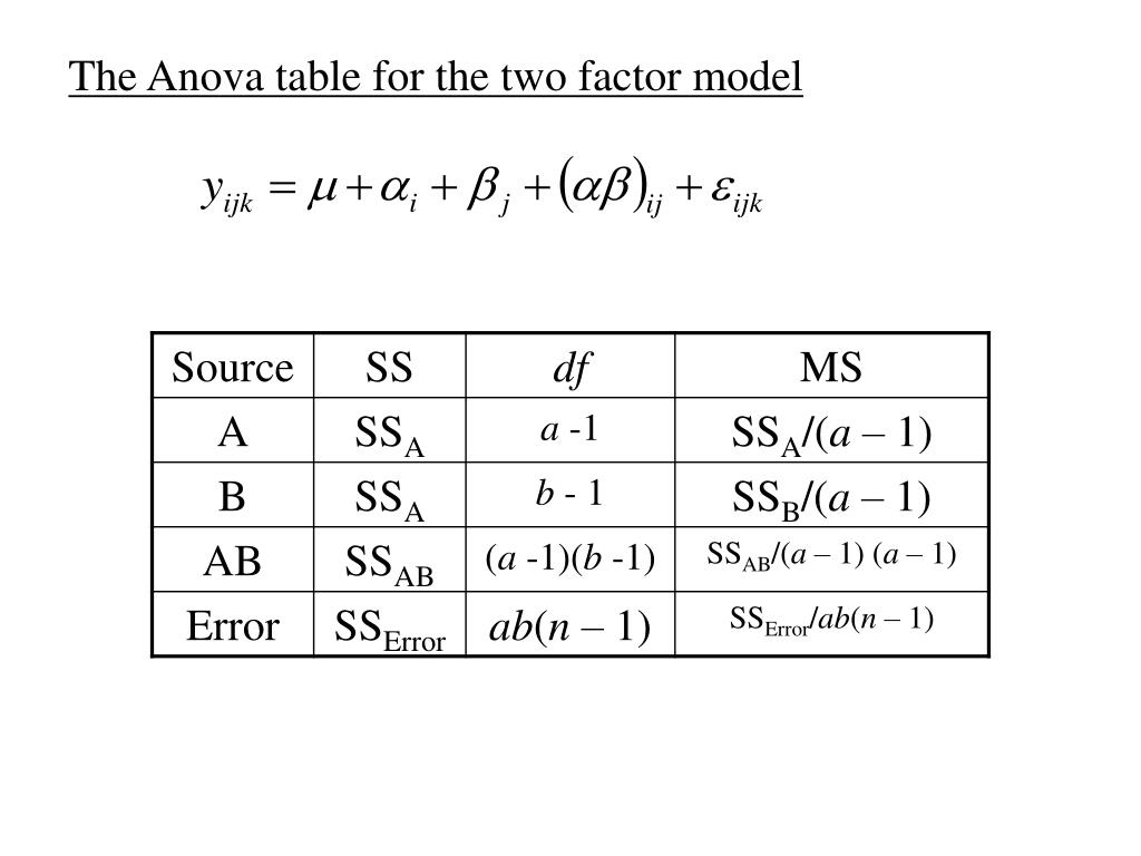
A Two-Way ANOVA evaluates the impact of two independent categorical factors (Factor A with $a$ levels and Factor B with $b$ levels) on a continuous outcome variable. When cell sizes are equal (a balanced design with $n$ observations per cell), total variance is partitioned into four distinct elements: Factor A, Factor B, Factor A $\times$ Factor B Interaction, and Residual Error.
Formulas for Balanced Two-Way ANOVA
For a design with $a$ levels of Factor A, $b$ levels of Factor B, and $n$ replicates per cell, the total number of observations is $N = a \cdot b \cdot n$.
Let:
- $T_{i\cdot\cdot}$: Sum of all observations at level $i$ of Factor A.
- $T_{\cdot j\cdot}$: Sum of all observations at level $j$ of Factor B.
- $T_{ij\cdot}$: Sum of all observations in cell $(i, j)$.
- $T_{\cdot\cdot\cdot}$: Grand total of all observations.
Correction Factor ($CF$)
$$CF = \frac{T_{\cdot\cdot\cdot}^2}{a \cdot b \cdot n}$$
Sum of Squares ($SS$)
Total Sum of Squares: $$SS_{\text{Total}} = \sum_{i=1}^{a} \sum_{j=1}^{b} \sum_{k=1}^{n} X_{ijk}^2 - CF$$
Factor A Sum of Squares: $$SS_A = \frac{\sum_{i=1}^{a} T_{i\cdot\cdot}^2}{b \cdot n} - CF$$
Factor B Sum of Squares: $$SS_B = \frac{\sum_{j=1}^{b} T_{\cdot j\cdot}^2}{a \cdot n} - CF$$
Subtotals Sum of Squares (Cells): $$SS_{\text{Subtotals}} = \frac{\sum_{i=1}^{a} \sum_{j=1}^{b} T_{ij\cdot}^2}{n} - CF$$
Interaction Sum of Squares ($SS_{AB}$): $$SS_{AB} = SS_{\text{Subtotals}} - SS_A - SS_B$$
Error Sum of Squares ($SS_{\text{Error}}$): $$SS_{\text{Error}} = SS_{\text{Total}} - SS_{\text{Subtotals}} = SS_{\text{Total}} - (SS_A + SS_B + SS_{AB})$$
Degrees of Freedom ($DF$)
- $DF_A = a - 1$
- $DF_B = b - 1$
- $DF_{AB} = (a - 1)(b - 1)$
- $DF_{\text{Error}} = a \cdot b \cdot (n - 1)$
- $DF_{\text{Total}} = a \cdot b \cdot n - 1 = N - 1$
Mean Squares ($MS$)
- $MS_A = \frac{SS_A}{a - 1}$
- $MS_B = \frac{SS_B}{b - 1}$
- $MS_{AB} = \frac{SS_{AB}}{(a - 1)(b - 1)}$
- $MS_{\text{Error}} = \frac{SS_{\text{Error}}}{a \cdot b \cdot (n - 1)}$
$F$-Statistics
Each source term is tested against Mean Square Error:
- Main Effect of A: $F_A = \frac{MS_A}{MS_{\text{Error}}}$
- Main Effect of B: $F_B = \frac{MS_B}{MS_{\text{Error}}}$
- Interaction Effect (A $\times$ B): $F_{AB} = \frac{MS_{AB}}{MS_{\text{Error}}}$
Two-Way ANOVA Summary Table (Balanced Design)
| Source of Variation | Sum of Squares ($SS$) | Degrees of Freedom ($DF$) | Mean Square ($MS$) | $F$-Ratio |
|---|---|---|---|---|
| Factor A | $SS_A$ | $a - 1$ | $MS_A = \frac{SS_A}{a - 1}$ | $F_A = \frac{MS_A}{MS_{\text{Error}}}$ |
| Factor B | $SS_B$ | $b - 1$ | $MS_B = \frac{SS_B}{b - 1}$ | $F_B = \frac{MS_B}{MS_{\text{Error}}}$ |
| Interaction ($A \times B$) | $SS_{AB}$ | $(a - 1)(b - 1)$ | $MS_{AB} = \frac{SS_{AB}}{(a - 1)(b - 1)}$ | $F_{AB} = \frac{MS_{AB}}{MS_{\text{Error}}}$ |
| Error (Within) | $SS_{\text{Error}}$ | $a \cdot b \cdot (n - 1)$ | $MS_{\text{Error}} = \frac{SS_{\text{Error}}}{DF_{\text{Error}}}$ | — |
| Total | $SS_{\text{Total}}$ | $a \cdot b \cdot n - 1$ | — | — |
Step-by-Step Worked Example: Calculating a One-Way ANOVA Table
To illustrate how these formulas operate in practice, consider an experiment comparing three different fertilizer formulations ($k = 3$) on plant crop yield.
Sample Data Set
- Group 1 (Fertilizer A): 10, 12, 14 ($n_1 = 3$)
- Group 2 (Fertilizer B): 16, 18, 20 ($n_2 = 3$)
- Group 3 (Fertilizer C): 22, 24, 26 ($n_3 = 3$)
Summary Totals and Means:
- Total observations $N = 3 + 3 + 3 = 9$
- Group 1: $T_{1\cdot} = 10 + 12 + 14 = 36$, $\bar{X}_{1\cdot} = 12$
- Group 2: $T_{2\cdot} = 16 + 18 + 20 = 54$, $\bar{X}_{2\cdot} = 18$
- Group 3: $T_{3\cdot} = 22 + 24 + 26 = 72$, $\bar{X}_{3\cdot} = 24$
- Grand Total $T_{\cdot\cdot} = 36 + 54 + 72 = 162$
- Grand Mean $\bar{X}_{\cdot\cdot} = \frac{162}{9} = 18$
Step 1: Compute Sum of Squares
Calculate Correction Factor ($CF$): $$CF = \frac{T_{\cdot\cdot}^2}{N} = \frac{162^2}{9} = \frac{26244}{9} = 2916$$
Calculate Total Sum of Squares ($SS_{\text{Total}}$): Sum of squared raw scores: $$\sum \sum X_{ij}^2 = 10^2 + 12^2 + 14^2 + 16^2 + 18^2 + 20^2 + 22^2 + 24^2 + 26^2$$ $$\sum \sum X_{ij}^2 = 100 + 144 + 196 + 256 + 324 + 400 + 484 + 576 + 676 = 3156$$ $$SS_{\text{Total}} = 3156 - 2916 = 240$$
Calculate Between-Groups Sum of Squares ($SS_{\text{Between}}$): $$SS_{\text{Between}} = \left( \frac{36^2}{3} + \frac{54^2}{3} + \frac{72^2}{3} \right) - 2916$$ $$SS_{\text{Between}} = \left( \frac{1296}{3} + \frac{2916}{3} + \frac{5184}{3} \right) - 2916$$ $$SS_{\text{Between}} = (432 + 972 + 1728) - 2916 = 3132 - 2916 = 216$$
Calculate Within-Groups Sum of Squares ($SS_{\text{Error}}$): $$SS_{\text{Error}} = SS_{\text{Total}} - SS_{\text{Between}} = 240 - 216 = 24$$
Step 2: Compute Degrees of Freedom
- $DF_{\text{Between}} = k - 1 = 3 - 1 = 2$
- $DF_{\text{Error}} = N - k = 9 - 3 = 6$
- $DF_{\text{Total}} = N - 1 = 9 - 1 = 8$
Step 3: Compute Mean Squares
- $MS_{\text{Between}} = \frac{SS_{\text{Between}}}{DF_{\text{Between}}} = \frac{216}{2} = 108$
- $MS_{\text{Error}} = \frac{SS_{\text{Error}}}{DF_{\text{Error}}} = \frac{24}{6} = 4$
Step 4: Compute the F-Ratio
$$F = \frac{MS_{\text{Between}}}{MS_{\text{Error}}} = \frac{108}{4} = 27$$
Final Calculated ANOVA Table
| Source of Variation | Sum of Squares ($SS$) | Degrees of Freedom ($DF$) | Mean Square ($MS$) | $F$-Ratio | $p$-value |
|---|---|---|---|---|---|
| Between Groups | 216 | 2 | 108 | 27.00 | $< 0.001$ |
| Within Groups (Error) | 24 | 6 | 4 | — | — |
| Total | 240 | 8 | — | — | — |
Statistical Interpretation: The critical $F$-value for $DF=(2, 6)$ at $\alpha = 0.05$ is approximately $5.14$. Because $F_{\text{calculated}} = 27.00 > 5.14$, we reject the null hypothesis and conclude that fertilizer formulations produce statistically significant differences in average crop yield.
Assumptions and Limitations in ANOVA Calculations
Applying ANOVA formulas validly requires meeting specific underlying statistical assumptions. Violations can distort $p$-values and inflate false positive rates.
- Assumptions of ANOVA
- Normality: Residuals must follow normal distribution
- Homogeneity of Variance: Group variances must be equal (Homoscedastic)
- Independence of Errors: Observations must be independent across samples
Core Statistical Assumptions
- Normality: Residuals within each treatment group should be approximately normally distributed. Minor departures can be tolerated due to the Central Limit Theorem, especially with larger sample sizes.
- Homogeneity of Variance (Homoscedasticity): The variances across comparing groups must be equal ($\sigma_1^2 = \sigma_2^2 = \dots = \sigma_k^2$). Tests such as Levene’s Test or Bartlett’s Test verify this assumption. If violated, corrections such as Welch's ANOVA should be used instead of standard ANOVA formulas.
- Independence: Observations within and across samples must be mutually independent. Dependent or repeated measures require alternate analytical procedures, such as a Repeated Measures ANOVA.
Handling Unbalanced Data
In Two-Way ANOVA, if group sizes ($n_{ij}$) are unequal across cells, traditional simple formulas for Sum of Squares do not add up cleanly to $SS_{\text{Total}}$ because terms become correlated. Software implementations resolve this using Type I, Type II, or Type III Sum of Squares:
- Type I (Sequential): Dependent on factor entry order in the model.
- Type II (Hierarchical): Evaluates main effects controlling for other main effects without interaction terms.
- Type III (Marginal/Orthogonal): Evaluates each factor effect adjusted for all other main effects and interactions. This is the standard method used by major statistical software packages (R, SAS, SPSS, Python statsmodels).
Technical Guidelines for Post-Hoc Analysis
An ANOVA $F$-test is omnibus: a statistically significant $F$-ratio indicates that at least two group means differ, but it does not specify which specific pairs differ.
When $H_0$ is rejected, post-hoc multiple comparison tests are applied:
- Tukey’s Honestly Significant Difference (HSD): Ideal for pairwise comparisons between all group means while controlling the family-wise error rate.
- Bonferroni Correction: A conservative approach for testing a pre-selected subset of group pairs.
- Dunnett’s Test: Used when comparing multiple treatment groups against a single control group.
Frequently Asked Questions
What is the relationship between SS, DF, and MS in an ANOVA table?
Mean Square ($MS$) is calculated by dividing Sum of Squares ($SS$) by its corresponding Degrees of Freedom ($DF$), expressed as $MS = \frac{SS}{DF}$. This calculation standardizes variance estimates across groups of different sample sizes and constraints.
Why is an ANOVA table used instead of multiple t-tests?
Running multiple independent $t$-tests on three or more groups causes cumulative inflation of the Type I error rate ($\alpha$). For $k$ groups, there are $\frac{k(k-1)}{2}$ unique pairs. Performing multiple tests raises the overall false positive rate far above $\alpha=0.05$. An ANOVA table evaluates all group means simultaneously in a single test at the specified significance level.
Can Mean Square Error (MSE) ever be negative?
No. Sum of Squares ($SS$) is calculated by summing squared real numbers, which guarantees non-negative values. Because Degrees of Freedom ($DF$) is always positive, Mean Square Error ($MS = \frac{SS}{DF}$) must also be non-negative.
How do you find the critical F-value for an ANOVA table?
The critical $F$-value is obtained from an $F$-distribution table or statistical computing software using three inputs: the chosen significance level $\alpha$ (typically $0.05$), the numerator degrees of freedom ($DF_{\text{Between}}$ or $DF_{\text{Factor}}$), and the denominator degrees of freedom ($DF_{\text{Error}}$).
What is the difference between One-Way and Two-Way ANOVA formulas?
One-Way ANOVA formulas split total variance into two sources: Between Groups (Treatment) and Within Groups (Error). Two-Way ANOVA formulas split total variance into four sources: Factor A, Factor B, Factor A $\times$ Factor B Interaction, and Residual Error.
Practical Recommendations & Next Steps
When analyzing experimental data using ANOVA formulas:
- Verify Assumptions First: Check for normality using the Shapiro-Wilk test and homoscedasticity using Levene’s test before relying on $F$-test statistical conclusions.
- Select the Right SS Type for Unbalanced Data: If working with unequal cell sizes in multi-factor designs, use Type III Sum of Squares via statistical software rather than manual hand-calculation formulas.
- Follow Up with Post-Hoc Tests: If your ANOVA yields a significant $F$-statistic ($p < 0.05$), execute post-hoc pairwise procedures like Tukey’s HSD to identify exact group differences.
- Report Standard Metrics: When documenting ANOVA results in technical reports, present the complete table containing $SS$, $DF$, $MS$, $F$-value, and precise $p$-value, along with calculated effect sizes such as Eta-squared ($\eta^2 = \frac{SS_{\text{Between}}}{SS_{\text{Total}}}$).