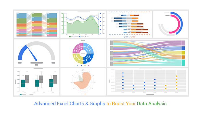
Excel advanced charts transform complex numerical datasets into dynamic, high-impact visual stories through techniques like secondary axes, variable width columns, Gantt timelines, and scrollable interactive dashboards. By combining native chart elements with named ranges, formulas, and VBA, users can build presentations that respond instantly to changing underlying data without requiring external software.
Understanding the Scope of Advanced Charts in Excel
Basic Excel charts—such as standard column, line, and pie graphs—are often sufficient for showing simple trends or distributions. However, modern business reporting, engineering analysis, and financial modeling frequently demand visualizations that can handle multi-scale data, dynamic timeframes, or non-standard distributions. Advanced charting in Microsoft Excel bridges the gap between raw tables and executive-level dashboards by leveraging hidden data structures, calculated series, and custom formatting rules.
When evaluating when to use advanced charts over basic alternatives, consider the complexity of the narrative you need to communicate. If you need to display project timelines alongside resource allocation, compare metrics with vastly different numerical scales (such as revenue in millions versus profit margins in percentages), or create self-updating dashboards that users can filter via form controls, standard single-series templates will fall short. Advanced techniques allow you to manipulate the underlying data source so that Excel’s rendering engine produces multi-layered, interactive outputs.
Core Prerequisites and Data Preparation
Before constructing any advanced chart, the underlying data must be structured with absolute consistency. Poorly organized datasets lead to broken series, incorrect category labels, and corrupted visualizations when filters or dynamic ranges are applied.
Data Structure Best Practices
- Header Rows: Ensure every column has a unique, descriptive text header. Avoid merged cells within the data range, as they break Excel's automatic range detection.
- Continuous Ranges: Keep your active data contiguous. Blank rows or columns inside a chart data range can cause Excel to split series or misinterpret data boundaries.
- Consistent Date Formats: When building timelines or time-series charts, verify that all date values use uniform serial numbers recognized by Excel rather than text-formatted strings.
Dynamic Ranges Using INDEX and OFFSET
To ensure your charts update automatically when rows or columns are added, you should define dynamic named ranges using formulas. For instance, combining the COUNTA and OFFSET functions allows a named range to expand or contract based on the number of populated cells:
=OFFSET(Sheet1!$A$2, 0, 0, COUNTA(Sheet1!$A:$A)-1, 1)
By referencing these named ranges in the Select Data Source dialog box instead of static cell references (e.g., Sheet1!$A$2:$A$100), your advanced charts will scale seamlessly as your database grows.
Essential Advanced Chart Types and Construction Techniques
Mastering advanced charts requires familiarity with specialized graph structures designed to solve specific analytical challenges. Below are four of the most powerful advanced charting techniques used in professional environments.
1. The Two-Axis (Combination) Chart
When comparing metrics with different scales—such as sales volume (units sold in the thousands) and profit margin (percentages)—plotting them on the same axis renders the smaller metric flat and unreadable.
Step-by-Step Implementation:
- Highlight your complete dataset, including headers for both series.
- Go to the Insert tab, click Recommended Charts, navigate to the All Charts tab, and select Combo.
- For the series representing the smaller scale (e.g., profit margin), check the box for Secondary Axis.
- Change the chart type for the primary series to a Clustered Column and the secondary series to a Line with Markers.
- Click OK to generate the chart, then format the axis bounds to ensure zero baseline alignment where appropriate.
2. The Gantt Chart (Project Management Scheduling)
Excel does not have a native "Gantt chart" button, but you can easily build one by transforming a stacked bar chart.
Step-by-Step Implementation:
- Organize your data with columns for Task Name, Start Date, and Duration (number of days).
- Insert a Stacked Bar Chart. Excel will initially plot both the start date and the duration.
- Click on the first series (the start dates, typically colored blue) and format them to have No Fill and No Line so they become invisible, acting as spacing offsets.
- Reverse the order of the vertical category axis by right-clicking it, selecting Format Axis, and checking Categories in reverse order.
- Format the date axis by adjusting minimum and maximum bounds to match your project's start and end date serial numbers.
3. The Waterfall Chart (Financial Bridge Analysis)
Waterfall charts illustrate how an initial value is affected by a series of positive and negative intermediate values, culminating in a net final balance. While Excel introduced a native waterfall chart type in modern versions, building a custom stacked column waterfall provides greater control over formatting and floating steps.
Custom Construction Method:
- Set up columns for Base, Invisible Filler (calculated to push floating columns up or down), and Visible Value.
- Plot as a Stacked Column Chart.
- Format the Invisible Filler series to have No Fill.
- Color-code the remaining visible columns using green for positive variances and red for negative subtotals.
4. Scrollable and Interactive Charts
For dashboards with extensive historical data, displaying all data points at once creates visual clutter. By integrating a scroll bar form control with INDEX formulas, you can create a chart that displays a fixed window of data (e.g., trailing 12 months) that users can scroll through.
Implementation Summary:
- Insert a Scroll Bar from the Developer tab (Insert > Form Controls).
- Link the scroll bar to a control cell (e.g.,
Sheet1!$Z$1) and set minimum/maximum parameters based on your total row count. - Create a helper table that uses the
INDEXfunction, referencing the scroll bar's linked cell to dynamically pull a subset of rows from the master database. - Base your chart exclusively on this small helper table.
| Chart Type | Primary Business Use Case | Key Configuration Steps | Common Pitfall to Avoid |
|---|---|---|---|
| Combo Chart | Comparing metrics of different scales (e.g., Volume vs. Rate) | Assign secondary series to secondary axis; change chart types per series. | Forgetting to align zero baselines, which misleads visual comparisons. |
| Gantt Chart | Project schedules, task timelines, and resource tracking | Format start-date series as invisible; reverse category axis order. | Leaving default date serial numbers unformatted on the horizontal axis. |
| Waterfall Chart | Financial variance analysis, P&L bridges, and inventory audits | Use invisible stack columns as spacers beneath floating value columns. | Incorrectly calculating floating filler formulas for negative subtotals. |
| Scrollable Chart | Long-term trend analysis on space-constrained executive dashboards | Link a Form Control scroll bar to dynamic helper formulas using INDEX. |
Setting scroll bar maximum values beyond actual data length, causing #REF! errors. |
Formatting and Design Principles for Professional Output
Advanced functionality is valuable only if the resulting visualization communicates information clearly. Poor formatting undermines even the most sophisticated data models.
Eliminating Chart Clutter (Chart Junk)
Coined by Edward Tufte, the term "chart junk" refers to all visual elements in charts that are not necessary to comprehend the data.
- Gridlines: Remove vertical gridlines entirely. Keep horizontal gridlines faint and sparse only if exact value reading is required.
- Borders and Backgrounds: Remove heavy outer borders from the chart area. Let the chart breathe by matching its background to the surrounding worksheet or keeping it clean white.
- Legends: If your chart contains only one or two clear series, eliminate the legend entirely and use a descriptive chart title that clarifies the data units.
Color Theory and Accessibility
- Semantic Coloring: Use colors with established psychological meaning—such as green for positive growth and red for negative variance—only when appropriate. Avoid using red and green adjacent to one another without pattern fills or direct labeling, as this alienates color-blind readers.
- Restraint: Limit your palette to two or three related tones for general data series, reserving high-saturation accent colors exclusively to draw attention to outlier data points.
Troubleshooting Common Advanced Chart Errors
When building complex charts, users frequently encounter rendering errors or unexpected visual bugs. Below are solutions to the most frequent issues.
1. The Disappearing Series Issue
If adding a new series causes an existing series to vanish or corrupts the horizontal axis, Excel has likely misinterpreted whether your data is arranged in rows or columns.
- Solution: Right-click the chart, select Select Data, and verify the orientation in the Switch Row/Column menu. Ensure your series names are explicitly selected in the Legend Entries box rather than left for Excel to guess automatically.
2. Hidden Data and Zero Values Showing as Dips
By default, Excel plots empty cells as zeros, which can ruin trend lines or create misleading drops in line and area charts.
- Solution: Click on the chart, go to Select Data, and click the Hidden and Empty Cells button in the bottom-left corner. Change the setting from "Zero" to "Span data nulls" (for line charts) or "Leave blank". If using formulas, return
NA()instead of empty strings ("") to force Excel to ignore those data points entirely.
3. Axis Scaling Resets Upon Data Refresh
When dynamic named ranges update, Excel occasionally resets custom axis minimum and maximum bounds back to automatic settings, throwing off carefully formatted visual proportions.
- Solution: Lock down your axis bounds manually in the Format Axis task pane, or write a short Worksheet Change event in VBA that recalculates optimal bounds upon data updates.
Frequently Asked Questions
How do I make an Excel chart update automatically when I add new data?
You can make an Excel chart update automatically by converting your source data range into an official Excel Table (press Ctrl + T) or by defining dynamic named ranges using formulas like OFFSET and COUNTA. When new rows are appended, tables and dynamic ranges expand automatically, and the chart's data source reference absorbs the additions without manual re-selection.
Can I combine a column chart and a line chart in Excel?
Yes, this is achieved using a Combo Chart. Select your data, navigate to Insert > Recommended Charts > All Charts > Combo, and assign different chart types to each individual series. You can also assign series to a secondary vertical axis if their numerical ranges differ significantly.
Why is my Gantt chart showing bars starting from the wrong date?
This usually happens because Excel interprets the first series (the start date) as visible data rather than a transparent offset. To fix this, click the start-date series in the chart, open the Format Data Series pane, set Fill to "No fill" and Border to "No line". Additionally, check that your date axis minimum bound matches the correct Excel date serial number.
How do I plot data with completely different scales on the same chart?
To plot disparate scales—such as revenue in millions alongside customer satisfaction scores as percentages—use a secondary axis. In a Combo Chart setup, check the Secondary Axis box for the series with the smaller numerical values. Ensure both axes start at logical baselines to prevent the visual comparison from distorting reader interpretation.
Next Actions and Further Practice
To solidify your mastery of advanced charting in Excel, begin by auditing an existing static report or dashboard within your workflow. Identify areas where users must mentally calculate variances or toggle between disconnected tables, and replace those sections with a dynamic combination chart or a scrollable trend window. Practice building named ranges in a blank workbook before attempting to retrofit them onto legacy spreadsheets. For complex financial modeling or large-scale operational dashboards, explore pairing these advanced visual techniques with PivotCharts and slicers for an even greater degree of interactivity.