To build an IF function with three conditions in Excel, you can use a nested IF statement for sequential tiers, apply the modern IFS function for cleaner multi-test evaluation, or combine IF with AND/OR logical operators to test three simultaneous criteria within a single logical statement.
Understanding Multi-Condition Logic in Microsoft Excel
The standard Microsoft Excel IF function evaluates a logical premise, returning one value if the statement evaluates to TRUE and another if it evaluates to FALSE. The fundamental syntax for the base function is:
=IF(logical_test, value_if_true, [value_if_false])
In day-to-day data modeling, financial reporting, and inventory management, business logic regularly exceeds a simple binary check. Real-world tasks frequently demand testing three distinct conditions. When handling three conditions, the structure of your formula depends entirely on the logical relationship between those criteria:
- Mutually Exclusive Sequential Logic (Categorization or Tiering): You have three conditions that yield different results at different stages (for example, grading scales, commission tiers, or project status stages).
- Compound Conjunction (All Must Be Met): You need three separate criteria to all resolve to
TRUEsimultaneously before a single positive action triggers. - Compound Disjunction (Any Can Be Met): You need at least one of three separate conditions to resolve to
TRUEto trigger an outcome.
Understanding the difference between sequential evaluation and compound testing prevents formula construction errors, reduces calculation overhead, and ensures workbooks remain scalable.
Method 1: The Classic Nested IF Statement
The nested IF statement represents the traditional method for evaluating multiple conditions in Microsoft Excel. It works by placing a secondary IF statement inside the value_if_false or value_if_true argument of an existing IF function.
Nested IF formulas are universally backwards-compatible with every version of Microsoft Excel, including Excel 2003, Excel 2007, and legacy spreadsheet software that cannot process modern dynamic array functions.
The Underlying Syntax
When evaluating three conditions where each condition yields its own result, two nested IF functions are linked together:
=IF(Condition_1, Result_1, IF(Condition_2, Result_2, IF(Condition_3, Result_3, Default_Result)))
In this architecture, Excel evaluates Condition_1. If it is true, the formula returns Result_1 and immediately halts execution. If Condition_1 is false, Excel proceeds to the second argument, evaluating Condition_2. This waterfall execution continues until a condition evaluates to TRUE or the formula reaches the final Default_Result.
Practical Business Example: Tiered Sales Commission
Consider an organization calculating commission rates based on individual sales volume in cell B2:
- Sales of $50,000 or more earn a 10% commission.
- Sales of $30,000 to $49,999 earn a 7% commission.
- Sales of $15,000 to $29,999 earn a 4% commission.
- Sales under $15,000 earn 0% commission.
The nested formula is written as follows:
=IF(B2>=50000, 0.10, IF(B2>=30000, 0.07, IF(B2>=15000, 0.04, 0)))
Critical Rule: The Order of Evaluation
When constructing a nested IF statement with numerical thresholds, you must arrange your conditions in strict descending or ascending order.
If you write =IF(B2>=15000, 0.04, IF(B2>=30000, 0.07, IF(B2>=50000, 0.10, 0))), any sales value above $15,000—including an entry of $65,000—will trigger the first logical test (B2>=15000). Excel evaluates this initial check as TRUE, issues the 0.04 result, and never inspects the subsequent 7% or 10% thresholds. To prevent false classifications, always evaluate the most restrictive boundary first when working downward, or the lowest boundary first when working upward with less-than (<) operators.
Method 2: The Modern IFS Function
Introduced in Excel 2019 and standard across Microsoft 365, Excel for the Web, and modern perpetual editions, the IFS function eliminates the syntactical complexity of nesting multiple parentheses. Instead of embedding opening and closing IF calls inside one another, IFS reads conditions and values in paired arguments.
The Underlying Syntax
The syntax for IFS runs linearly across logical pairs:
=IFS(logical_test1, value_if_true1, [logical_test2, value_if_true2], [logical_test3, value_if_true3], ...)
The function accepts up to 127 condition/value pairs. Unlike the standard IF function, IFS lacks a native built-in value_if_false argument. To supply a default outcome if none of the three conditions are satisfied, you establish a final condition evaluated as the literal boolean value TRUE.
Practical Business Example: Project Urgency Classification
Suppose project tasks listed in an operations spreadsheet need risk tags assigned according to days past due, stored in cell C2:
- More than 30 days past due: "Critical"
- 15 to 30 days past due: "Elevated"
- 1 to 14 days past due: "Standard"
- 0 or negative days (on schedule): "On Track"
Using IFS, the formula is constructed without nested brackets:
=IFS(C2>30, "Critical", C2>=15, "Elevated", C2>=1, "Standard", TRUE, "On Track")
How the Default Catch-All Works
In the formula above, Excel examines each argument sequentially:
- If cell
C2contains 45,C2>30isTRUE, returning "Critical". - If cell
C2contains 20, the first test fails, butC2>=15isTRUE, returning "Elevated". - If cell
C2contains 5, the first two tests fail, butC2>=1isTRUE, returning "Standard". - If cell
C2contains 0, all three numerical checks fail. Excel encounters the finalTRUEcondition, which by definition evaluates as affirmative, returning the catch-all string "On Track".
If you omit the TRUE, "On Track" argument pair and none of the three primary conditions are met, Excel returns a #N/A error.
Method 3: Combining IF with Logical Operators (AND / OR)
When your analytical objective is not assigning three different tiers, but rather checking whether three conditions are satisfied at the same time—or whether any one of three separate parameters is satisfied—nesting is unnecessary. Instead, pair a single outer IF statement with the AND or OR logical functions.
Scenario A: All Three Conditions Must Be True (IF + AND)
The AND function accepts multiple logical criteria and returns TRUE only if every single argument evaluates to affirmative. If even one test returns FALSE, the entire AND block evaluates to FALSE.
Syntax:
=IF(AND(Condition_1, Condition_2, Condition_3), Value_if_All_True, Value_if_Any_False)
Practical Example: Performance Bonus Approval
To qualify for an annual executive bonus, an employee must satisfy three business hurdles simultaneously:
- Total Sales (cell
B2) must exceed $100,000. - Customer Satisfaction Score (cell
C2) must be at least 90%. - Total Compliance Violations (cell
D2) must equal 0.
The formula tests all three metrics within a single execution:
=IF(AND(B2>100000, C2>=0.90, D2=0), "Eligible", "Not Eligible")
Because AND acts as an absolute gatekeeper, an employee with $250,000 in sales and a 98% satisfaction rating will still receive "Not Eligible" if their compliance violations figure equals 1.
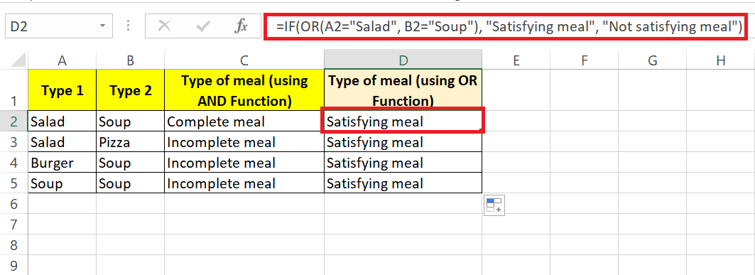
Scenario B: Any One of Three Conditions Can Be True (IF + OR)
The OR function tests multiple conditions and returns TRUE if at least one argument resolves to affirmative. It only returns FALSE if every listed condition fails.
Syntax:
=IF(OR(Condition_1, Condition_2, Condition_3), Value_if_At_Least_One_True, Value_if_All_False)
Practical Example: Warehouse Safety Inspection Flag
A storage facility manager must flag a pallet location in cell E2 for safety inspection if:
- Pallet Weight (cell
A2) exceeds 2,500 pounds, OR - Storage Duration (cell
B2) exceeds 180 days, OR - Structural Integrity Check (cell
C2) is marked "Damaged".
The formula is structured as:
=IF(OR(A2>2500, B2>180, C2="Damaged"), "Audit Required", "Approved")
If any single parameter matches the risk threshold, the formula immediately triggers the "Audit Required" protocol.
Scenario C: Mixed Logic (Combining AND and OR)
You can also nest AND and OR functions within the logical test of an IF statement to manage advanced multi-condition criteria.
For instance, an organization may approve loan financing if:
- Credit Score (cell
B2) is greater than 700, AND - Income (cell
C2) exceeds $50,000, AND - Either Years Employed (cell
D2) is greater than 2 OR Debt-to-Income Ratio (cellE2) is under 35%.
The formula combines these relationships cleanly:
=IF(AND(B2>700, C2>50000, OR(D2>2, E2<0.35)), "Approved", "Declined")
Comparison of the Three Methods
Selecting the correct formula architecture depends on your version of Excel, workbook maintainability goals, and the structure of your logic.
| Method | Best Use Case | Excel Compatibility | Syntax Complexity | Maintenance Risk |
|---|---|---|---|---|
| Nested IF | Sequential categories or tiering when backwards compatibility is strictly required. | All versions (Excel 97 through Microsoft 365) | High (requires matching multiple closing parentheses) | High (difficult to read and update when rules change) |
| IFS Function | Sequential categories or multi-branch logic in modern spreadsheet environments. | Excel 2019, Excel 2021, Microsoft 365, Excel Web | Moderate (linear pairs, no nested parentheses) | Low (clean structure; easily expanded with new pairs) |
| IF + AND / OR | Checking whether all three conditions or any of three conditions are met for a single outcome. | All versions (Excel 97 through Microsoft 365) | Low to Moderate (standard grouping) | Very Low (standardized logical tests inside one IF) |
Alternative Solutions for Complex Logic
While IF and IFS handle three conditions effectively, expanding beyond three or four conditions with standard logical functions can introduce formula bloat. When scale increases, consider two reliable alternatives:
1. The SWITCH Function
When three conditions evaluate an exact match against the same cell expression, the SWITCH function is cleaner than nested IF or IFS:
=SWITCH(A2, "North", 0.05, "South", 0.07, "West", 0.06, 0.04)
This formula inspects the region in A2. If it equals "North", it returns 5%; if "South", 7%; if "West", 6%; otherwise, it defaults to 4%. It avoids repeating the target cell address A2 across every check.
2. Lookup Tables with XLOOKUP or VLOOKUP
For sliding scales such as tax brackets, discount schedules, or performance scores, hardcoding numbers into nested IF statements is poor spreadsheet design. It exposes models to maintenance errors whenever business rates shift.
Instead, build a separate reference table and deploy an approximate match lookup:
=XLOOKUP(B2, Table_Tiers[SalesMin], Table_Tiers[Rate], 0, -1)
Using lookup models ensures you update assumptions in a single cell on a assumptions tab, rather than editing complex formulas across thousands of rows.
Best Practices for Building and Auditing Multi-Condition Formulas
Writing complex formulas requires structured habits to prevent logical mistakes and workbook corruption. Follow these core guidelines:
Format Formulas with In-Cell Line Breaks
When formulas expand across multiple tests, reading them horizontally across the Formula Bar invites syntax errors. Insert line breaks directly inside the formula by pressing Alt + Enter on Windows (or Option + Command + Enter on Mac). Excel ignores structural whitespace inside formulas:
=IF(B2>=50000, 0.10,
IF(B2>=30000, 0.07,
IF(B2>=15000, 0.04, 0)))
This formatting allows you to review individual logic branches vertically, much like writing structured code in Python or SQL.
Use the "Evaluate Formula" Tool
If a multi-condition formula yields an unexpected result, use Excel's step-by-step diagnostic tool:
- Select the cell displaying the questionable result.
- Navigate to the Formulas tab on the Excel Ribbon.
- In the Formula Auditing group, select Evaluate Formula.
- Click Evaluate repeatedly to watch Excel calculate each conditional expression step by step. This instantly reveals which logical argument returned
FALSEor triggered early.
Lock Reference Cells with Absolute References
If your conditional checks compare data against static input cells (such as standard commission percentages stored in header cells like $F$1, $F$2, $F$3), always anchor those references using absolute references (the $ symbol). Pressing F4 while drafting locks the column and row coordinates, preventing referenced cells from shifting down when you drag the formula across an entire table column.
Common Errors and Troubleshooting
When building three-condition IF formulas, spreadsheet authors frequently encounter four predictable errors:
1. The #VALUE! Error
- The Cause: Occurs most often when mathematical operators (such as
>,<,=) attempt to evaluate an incorrect data type, or when an invalid argument count is passed to a logical operator. - The Fix: Confirm that target cells contain true numeric values rather than numbers formatted as text. Text values imported from enterprise databases frequently contain non-breaking spaces that prevent mathematical evaluation.
2. The #N/A Error in the IFS Function
- The Cause: In an
IFSformula, every listed logical test evaluated toFALSE, and the formula lacked a catch-all argument. - The Fix: Ensure your final argument pair inside the
IFSfunction is set toTRUE, "Your_Default_Value".
3. Unexpected Outputs from Incorrect Comparison Sequences
- The Cause: If your formula checks
>=1000before checking>=5000, any input value of 6000 satisfies the initial>=1000test. Excel fires the first true result and terminates calculation. - The Fix: Reorder your arguments. For greater-than checks (
>,>=), begin with the highest numerical threshold and work downward. For less-than checks (<,<=), begin with the lowest threshold and work upward.
4. Formula Closing Parenthesis Mismatch
- The Cause: A nested IF statement requires exactly as many closing parentheses at the end of the expression as there are opening
IFstatements. - The Fix: Pay close attention to Excel's color-coded bracket highlights when editing the formula. The final closing parenthesis is always black. If your formula ends with a purple, green, or red parenthesis, you have missed a closing marker.
Frequently Asked Questions
Can I mix AND and OR operators inside an IFS function?
Yes. You can place an AND or OR function inside any logical test argument of an IFS statement. For example, =IFS(AND(A2="Complete", B2="Approved"), "Closed", OR(A2="Pending", B2="Pending"), "In Review", TRUE, "Unassigned") functions seamlessly. Each pair will evaluate its logical statement, including multi-condition combinations, before returning the associated output.
How many conditions can an IF function support in Excel?
Historically, Excel 2003 supported nesting up to 7 layers of IF statements. Modern editions of Microsoft Excel (from Excel 2007 onward) support up to 64 nested IF levels. However, nesting more than three or four levels is considered poor practice because formulas become brittle and difficult to audit. For logic with more than four criteria, dynamic lookup functions like XLOOKUP or structured lookup tables are recommended.
Why is my IF formula returning the formula text instead of the calculated value?
This occurs if the cell was formatted as "Text" before the formula was entered, or if the formula was prefixed with an apostrophe ('). To fix this, change the cell number format to General on the Home tab, click inside the Formula Bar, and press Enter. Ensure the formula starts strictly with an equals sign (=).
What is the main difference between Nested IF and IFS?
The primary difference is syntactical structure and error handling. Nested IF requires wrapping subsequent IF( functions inside the false argument of previous ones, creating layered closing parentheses at the end. The IFS function organizes tests in flat, sequential pairs (condition1, value1, condition2, value2). Additionally, nested IF includes a standard value_if_false slot, whereas IFS requires an explicit TRUE, default_value entry to prevent #N/A errors when all conditions fail.
Can I use text comparisons with these multi-condition formulas?
Yes. Text comparisons can be used in any logical argument. Always enclose text criteria inside double quotation marks (for example, A2="Complete" or B2<>"Closed"). Excel comparisons are not case-sensitive by default; entering A2="california" will successfully match "California", "CALIFORNIA", or "california". If you require case-sensitive comparisons across your three conditions, wrap your logical test in the EXACT function, such as IF(EXACT(A2, "RegionA"), ...).
Next Steps and Recommended Actions
To implement these formulas effectively across your active spreadsheets:
- Audit Your Logical Structure: Determine whether your three conditions are mutually exclusive (requiring Method 1: Nested IF or Method 2: IFS) or co-dependent (requiring Method 3: IF with AND/OR).
- Standardize on Modern Functions When Possible: If your workbook is used strictly within modern business environments running Microsoft 365 or modern desktop versions, favor the
IFSfunction over nested IFs for improved readability. - Graduate to Lookups for Complex Scales: If your three conditions form part of a matrix that may expand to four, five, or more tiers in the future, migrate your criteria to an Excel Table and utilize
XLOOKUPwith an approximate match mode instead of hardcoding conditions into logic formulas.