The exponential distribution is a continuous probability distribution used to model the time or space between independent events occurring at a constant average rate. Common real-world examples include the lifespan of electronic components, the time between customer arrivals in a queue, and the intervals between radioactive decay events in physics.
In the realm of statistics and probability, few concepts are as foundational yet frequently misunderstood as the exponential distribution. By 2026, the proliferation of real-time data analytics and automated systems has made understanding this distribution more critical than ever. Whether you are an engineer predicting hardware failure, a business analyst optimizing staffing for a service desk, or a scientist studying natural phenomena, the exponential distribution provides the mathematical framework to turn randomness into actionable insights.
To master this concept, one must look beyond the formula and examine how it manifests in the physical and digital worlds. Below, we explore three distinct examples of the exponential distribution, analyzing the mathematical mechanics, the practical implications, and the unique "memoryless" property that defines this statistical model.
Defining the Exponential Distribution: Prerequisites for Modeling
Before examining specific examples, it is necessary to establish the technical parameters of the exponential distribution. It is characterized by a single parameter, denoted as lambda ($\lambda$), which represents the rate of the process. If we are measuring time, $\lambda$ is the average number of events per unit of time.
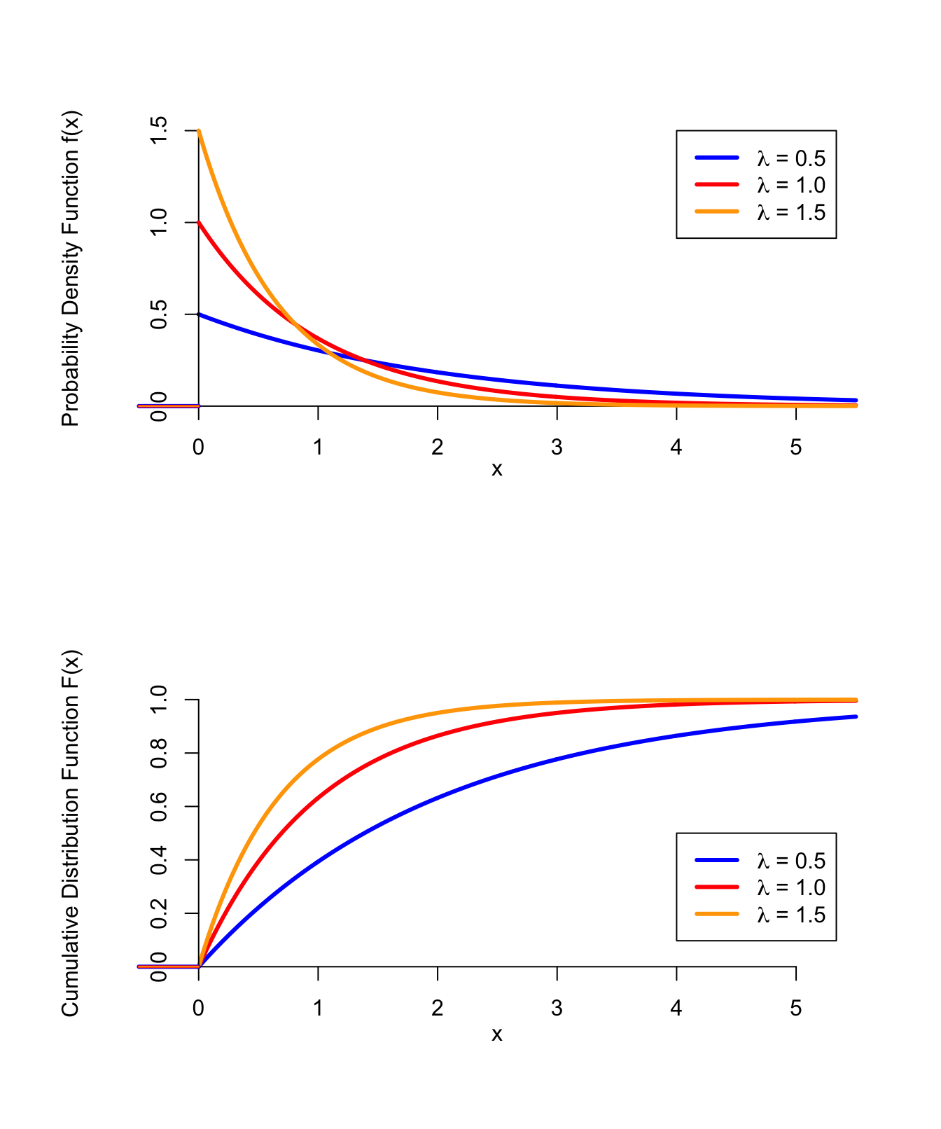
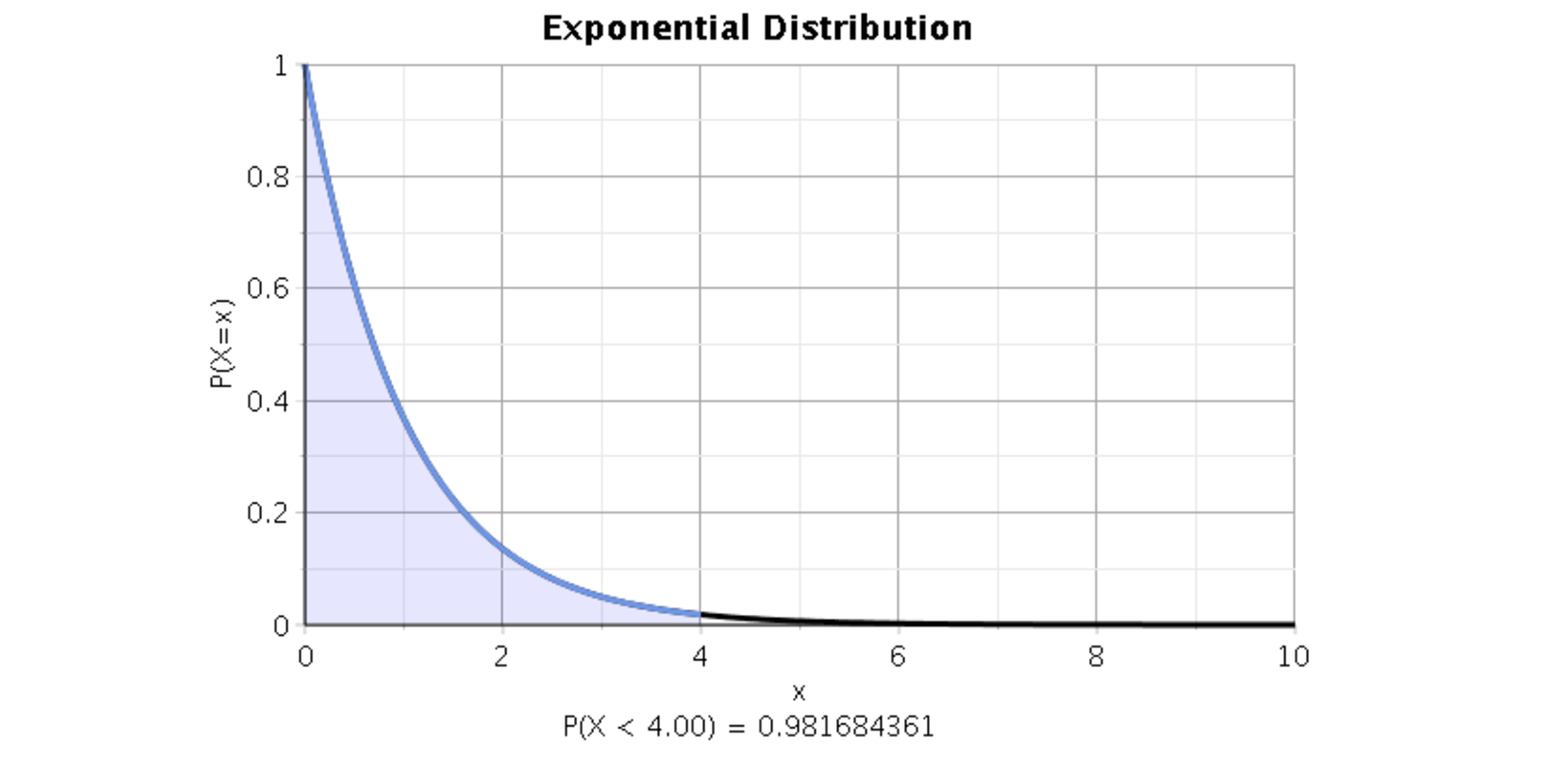
The Probability Density Function (PDF) is expressed as: $f(x; \lambda) = \lambda e^{-\lambda x}$ for $x \ge 0$
The Cumulative Distribution Function (CDF), which determines the probability that an event occurs within a certain timeframe, is: $F(x; \lambda) = 1 - e^{-\lambda x}$
Key characteristics include:
- The Mean (Expected Value): $1/\lambda$. If customers arrive at a rate of 10 per hour ($\lambda = 10$), the mean time between arrivals is $1/10$ of an hour, or 6 minutes.
- The Memoryless Property: This is the most unique feature of the distribution. It states that the probability of an event occurring in the next interval of time is independent of how much time has already passed. Mathematically: $P(T > s + t | T > s) = P(T > t)$.
Example 1: Reliability and Mean Time to Failure (MTTF) in Engineering
In industrial engineering and hardware manufacturing, the exponential distribution is the standard model for the "useful life" phase of a product. Most physical components follow what is known as the "Bathtub Curve." This curve describes three phases: infant mortality (high failure rate at the start), useful life (constant failure rate), and wear-out (increasing failure rate at the end). The exponential distribution specifically models the middle phase—the constant failure rate.
The Scenario: Server SSD Longevity
Consider a data center in 2026 utilizing high-capacity Solid State Drives (SSDs). Engineers have determined through stress testing that these drives have a constant failure rate of $\lambda = 0.0002$ failures per hour during their optimal operating window.
Mathematical Application
To find the probability that a specific drive will last at least 5,000 hours, we use the survival function $S(t) = e^{-\lambda t}$: $P(X > 5,000) = e^{-(0.0002)(5,000)} = e^{-1} \approx 0.368$
This tells the engineering team that there is a 36.8% chance a drive will survive past 5,000 hours without a random fault.
Why This Matters
By using this model, companies can calculate the Mean Time To Failure (MTTF). In this case, $MTTF = 1/0.0002 = 5,000$ hours. This metric is essential for setting warranty periods, determining how many spare parts to keep in stock, and scheduling preventive maintenance. If the distribution were not exponential—for instance, if the failure rate increased over time—the strategy would shift from "replace when broken" to "replace before the predicted wear-out."
Example 2: Service Queuing and Customer Inter-arrival Times
In the world of retail, banking, and digital infrastructure (like website server requests), the exponential distribution is the backbone of Queuing Theory. While the number of people who arrive in an hour follows a Poisson distribution, the time between those arrivals follows an exponential distribution.
The Scenario: Automated Pharmacy Kiosks
Imagine a high-traffic urban pharmacy in 2026 that uses automated kiosks for prescription pickup. On average, a new customer approaches a kiosk every 4 minutes. Here, the rate $\lambda$ is $1/4 = 0.25$ customers per minute.
Mathematical Application
A manager wants to know the probability that a new customer will arrive within 2 minutes of the previous one to ensure the kiosk interface resets quickly enough. Using the CDF: $P(X \le 2) = 1 - e^{-(0.25)(2)} = 1 - e^{-0.5} \approx 0.393$
There is a 39.3% probability that the next customer arrives in 2 minutes or less. Conversely, there is a 60.7% chance the kiosk will remain idle for more than 2 minutes.
The Role of Memorylessness in Service
One of the most counterintuitive aspects of this example is that if a kiosk has been empty for 10 minutes, the probability that a customer arrives in the next minute remains exactly the same as if a customer had just left. In reality, human behavior sometimes clusters, but for large-scale systems (like global web traffic), the exponential distribution provides a remarkably accurate approximation of these independent arrival events.
Example 3: Radioactive Decay and Particle Physics
In the natural sciences, the exponential distribution is not just a convenient model; it is a fundamental law of nature. Radioactive decay is perhaps the most perfect example of a memoryless process. An unstable atom does not "age"; the probability that it will decay in the next second is the same regardless of whether the atom has existed for an hour or a billion years.
The Scenario: Carbon-14 Dating
Carbon-14 is used by archaeologists to date organic materials. The rate of decay is constant for a given isotope. For Carbon-14, the decay rate $\lambda$ is approximately $1.209 \times 10^{-4}$ per year.
Mathematical Application
The relationship between the exponential distribution and "half-life" is a direct mathematical derivation. The half-life ($t_{1/2}$) is the time $t$ where the probability of survival is 0.5. $0.5 = e^{-\lambda t}$ $\ln(0.5) = -\lambda t$ $t_{1/2} = \ln(2) / \lambda$
For Carbon-14: $t_{1/2} \approx 0.693 / (1.209 \times 10^{-4}) \approx 5,730$ years.
Scientific Significance
This example demonstrates how the exponential distribution allows us to work backward from a known quantity of remaining substance to determine the time elapsed since the "start" of the process (e.g., the death of the organism). Because the decay is exponential, scientists can maintain high precision across vast timescales, provided they have a large enough sample size of atoms.
Comparative Analysis of Exponential Distribution Applications
To better understand how these examples differ in their practical implementation, the following table summarizes the key variables and use cases.
| Feature | Example 1: Hardware Reliability | Example 2: Service Queuing | Example 3: Radioactive Decay |
|---|---|---|---|
| Definition of $\lambda$ | Failures per unit of time (e.g., hours). | Arrivals per unit of time (e.g., minutes). | Decays per unit of time (e.g., years). |
| Primary Goal | Predicting lifespan and maintenance. | Optimizing wait times and staffing. | Determining age or safety of materials. |
| Key Metric | Mean Time to Failure (MTTF). | Average Inter-arrival Time. | Half-life ($t_{1/2}$). |
| Implication of Memorylessness | A used part is "as good as new" during its useful life. | Waiting 10 minutes doesn't make an arrival "due." | An old atom is no more likely to decay than a new one. |
| Common Industry | Manufacturing, Tech Infrastructure. | Retail, UX Design, Networking. | Geophysics, Medicine, Archaeology. |
Identifying and Avoiding Common Modeling Mistakes
While the exponential distribution is powerful, it is frequently misapplied. For a dataset to truly follow an exponential distribution, it must meet specific criteria.
1. The Constant Rate Assumption
The most common error is applying this distribution to a process where the rate $\lambda$ changes over time. For example, the time between car accidents at an intersection might be exponential over a 2-hour window on a Tuesday, but the rate $\lambda$ changes significantly between 3:00 AM and 5:00 PM (rush hour). If the rate is not constant, you are likely looking at a Non-Homogeneous Poisson Process, which requires more complex modeling.
2. Confusing Exponential with Poisson
A frequent point of confusion is the relationship between these two distributions.
- Poisson Distribution: Discrete. It counts the number of events in a fixed interval.
- Exponential Distribution: Continuous. It measures the time between those events. If you are asking "How many?" use Poisson. If you are asking "How long until?" use Exponential.
3. Misunderstanding the Memoryless Property
In human-centric scenarios, the memoryless property is often a "good enough" approximation rather than a literal truth. For example, in a "waiting for a bus" scenario, if the bus follows a strict schedule, the time between arrivals is not exponential. If you have already waited 10 minutes for a bus that comes every 15 minutes, you are objectively more likely to see it in the next 5 minutes. The exponential distribution only applies when events occur completely at random and independently.
Frequently Asked Questions
How does the exponential distribution relate to the Weibull distribution?
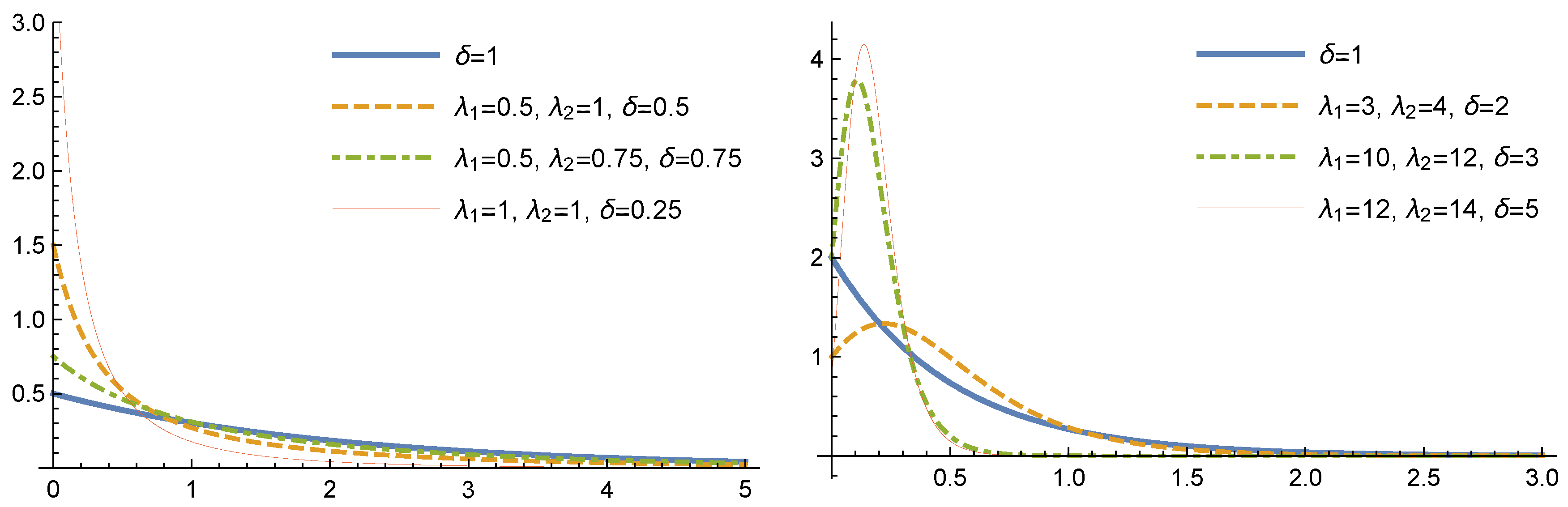
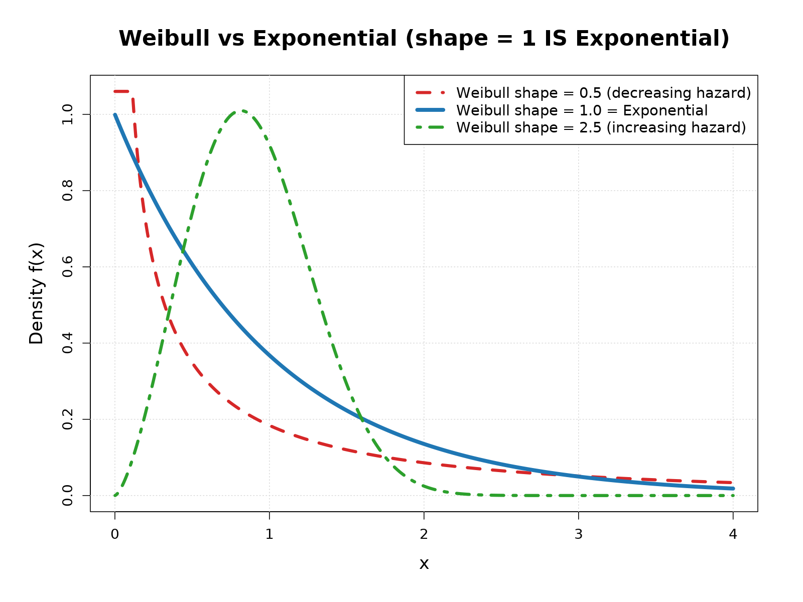
The Weibull distribution is essentially a more flexible version of the exponential distribution. While the exponential distribution assumes a constant failure rate, the Weibull distribution adds a "shape" parameter that allows for increasing or decreasing failure rates. In engineering, if a component shows signs of wear-and-tear (aging), the Weibull distribution is the superior choice.
Can the exponential distribution model the time between earthquakes?
To an extent, yes. Seismologists often use the exponential distribution to model the "inter-event" time between earthquakes in a specific region. However, this is a simplified model. Modern geophysics often uses the ETAS (Epidemic-Type Aftershock Sequence) model because earthquakes tend to trigger aftershocks, meaning the events are not strictly independent—a core requirement for a pure exponential distribution.
Why is the mean and standard deviation of an exponential distribution the same?
This is a unique mathematical property of the distribution. Both the mean ($\mu$) and the standard deviation ($\sigma$) are equal to $1/\lambda$. This means that the "spread" of the data is directly proportional to the average time between events. If the average time between customer arrivals increases, the variability or "uncertainty" of when the next customer will arrive increases by the same factor.
Is the exponential distribution always right-skewed?
Yes. The PDF of an exponential distribution always starts at its peak at $x=0$ and decays as $x$ increases. This results in a long "tail" to the right. This reflects the reality that while most intervals between events will be relatively short, there is always a small probability of a very long gap between events.
How do I calculate the median of an exponential distribution?
The median is not the same as the mean in a skewed distribution. For the exponential distribution, the median is calculated as $\ln(2) / \lambda$. Since $\ln(2)$ is approximately 0.693, the median is always about 69.3% of the mean. This means that in any exponential process, more than half of the intervals will be shorter than the average interval.
Practical Recommendation for Further Action
To apply these examples to your own data in 2026, the first step is to perform a Goodness-of-Fit test, such as the Kolmogorov-Smirnov test. This will help you determine if your observed inter-arrival times or failure data truly follow an exponential curve.
If you are working in Python, the scipy.stats.expon module is the industry standard for fitting these distributions. For those in business operations, begin by calculating your average rate ($\lambda$) over different time blocks to ensure that the "constant rate" assumption holds true before making staffing or inventory decisions. Understanding the nuances of the exponential distribution allows you to move beyond averages and start managing the inherent risks of random timing.