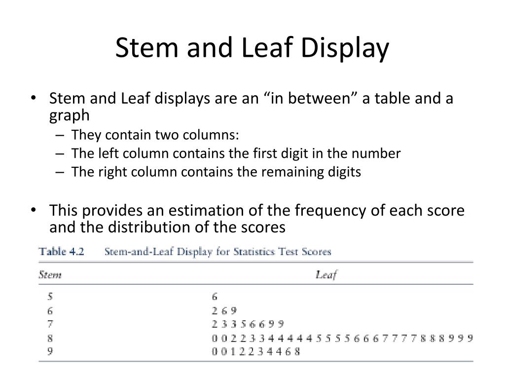
A stem and leaf display, also known as a stemplot, is a specialized table used to organize and visualize quantitative data by splitting each numerical value into a "stem" (the leading digit or digits) and a "leaf" (the final digit). These seven examples demonstrate how to handle various data types, including integers, decimals, and comparative datasets, while maintaining the integrity of individual data points.
Statistical visualization is a cornerstone of data interpretation, and the stem and leaf display remains one of the most effective tools for small to medium-sized datasets. Unlike histograms, which group data into intervals and lose the specific values of individual observations, a stemplot preserves every piece of information. In 2026, despite the ubiquity of automated dashboarding tools, the stem and leaf display is still a foundational requirement in academic curriculums and exploratory data analysis (EDA) for its ability to reveal distribution shape, central tendency, and outliers at a glance.
Understanding the Anatomy of a Stem and Leaf Plot
Before examining specific examples, it is necessary to understand the components of the display. Every stemplot consists of three primary parts: the stem, the leaf, and the key.
- The Stem: This represents the "leading" part of the data value. For a two-digit number like 45, the stem is 4. For a three-digit number like 128, the stem could be 12. Stems are listed vertically in a column, typically in ascending order.
- The Leaf: This is the "trailing" part of the value, usually the very last significant digit. In the number 45, the leaf is 5. If there are multiple values with the same stem, the leaves are listed horizontally next to that stem.
- The Key: This is the most critical element for interpretation. The key explains what the stem and leaf represents. For example, a key of "5 | 2 = 52 units" tells the reader that a stem of 5 and a leaf of 2 equals 52. Without a key, the reader wouldn't know if "5 | 2" meant 52, 5.2, or 0.52.
The primary goal of this format is to provide a visual "shape" to the data—much like a histogram turned on its side—while keeping the raw data accessible for calculations like the median or mode.
Example 1: Basic Single-Digit Leaves (Test Scores)
The most common application of a stemplot is tracking classroom performance or test scores. Consider a dataset of scores from a 100-point exam: 58, 67, 72, 75, 78, 81, 84, 84, 89, 91, 93, 98.
In this scenario, the tens digit serves as the stem, and the ones digit serves as the leaf.
Stem | Leaf 5 | 8 6 | 7 7 | 2 5 8 8 | 1 4 4 9 9 | 1 3 8
Key: 7 | 2 = 72%
This example highlights the distribution density. By looking at the plot, we can immediately see that the "80s" range is the most frequent (the mode interval), and the scores are slightly skewed towards the higher end. Because the leaves are ordered, finding the median is a simple matter of counting to the middle value.
Example 2: Decimal Data (Scientific Measurements)
Stem and leaf displays are not limited to whole numbers. They are frequently used in laboratory settings to track precise measurements, such as the pH levels of soil samples: 6.1, 6.3, 6.3, 6.8, 7.0, 7.2, 7.4, 7.4, 7.4, 7.9, 8.2.
To create this plot, the whole number becomes the stem, and the first decimal place becomes the leaf.
Stem | Leaf 6 | 1 3 3 8 7 | 0 2 4 4 4 9 8 | 2
Key: 7 | 0 = 7.0 pH
This display allows a researcher to see the clustering of samples. In this case, the majority of soil samples fall within the 7.0 to 7.9 range. It also identifies the value 8.2 as a potential outlier compared to the rest of the group, which could prompt further investigation into that specific sample.
Example 3: Large Datasets with Split Stems
When a dataset is large or highly concentrated within a small range, a standard stemplot can become "tall" and thin, providing little visual information. In these cases, we use split stems. Suppose we are measuring the pulse rates (beats per minute) of 20 individuals, where most scores fall between 60 and 80.
Data: 61, 62, 64, 66, 67, 68, 69, 70, 71, 71, 72, 73, 74, 75, 77, 78, 79, 81, 82, 85.
By splitting each stem into two (one for leaves 0–4 and one for leaves 5–9), we gain a clearer picture of the distribution.
Stem | Leaf 6 | 1 2 4 6 | 6 7 8 9 7 | 0 1 1 2 3 4 7 | 5 7 8 9 8 | 1 2 8 | 5
Key: 7 | 1 = 71 bpm
Splitting stems effectively doubles the "bins" of your distribution, similar to reducing the bin width in a histogram. It reveals that while the 70s are the most common range, the pulse rates are fairly evenly distributed between the high 60s and mid-70s.
Example 4: Double-Digit Leaves (Financial Data)
While leaves are typically single digits to maintain the visual "bar chart" effect, there are instances where double-digit leaves are used, especially when the precision of the second digit is vital, but the dataset is too small to justify rounding. This is common in financial reporting, such as daily stock price changes in cents.
Data: $1.15, $1.18, $1.22, $1.22, $1.35, $1.41, $1.49.
Stem | Leaf 1 | 15, 18, 22, 22, 35, 41, 49
Key: 1 | 15 = $1.15
Note: In modern statistical practice, it is generally preferred to round or truncate data to keep leaves as single digits (e.g., rounding $1.15 to $1.2). However, in specific technical audits where every cent matters, the double-digit leaf preserves the exact dataset while still providing a basic grouping structure.
Example 5: Back-to-Back Stemplot (Comparative Analysis)
The back-to-back stem and leaf display is one of the most powerful versions of this tool. It allows for the direct comparison of two different groups (e.g., Treatment vs. Control, or Male vs. Female) using a single shared stem.
Consider the heights (in inches) of two different groups of plants grown with different fertilizers.
- Fertilizer A: 12, 15, 18, 22, 25, 29
- Fertilizer B: 14, 17, 21, 23, 23, 26
Fertilizer A | Stem | Fertilizer B 8 5 2 | 1 | 4 7 9 5 2 | 2 | 1 3 3 6
Key: 2 | 1 = 21 inches
In this display, the leaves for Fertilizer A grow to the left, while the leaves for Fertilizer B grow to the right. This allows an analyst to see that Fertilizer A has a wider spread (from 12 to 29), whereas Fertilizer B is more tightly clustered in the low 20s.
Example 6: Three-Digit Data (Weight or Volume)
When dealing with larger numbers, such as the weights of packages in grams (e.g., 342, 345, 351, 358, 360), the "stem" can consist of the first two digits.
Stem | Leaf 34 | 2 5 35 | 1 8 36 | 0
Key: 35 | 1 = 351 grams
This approach is highly effective for technical specifications. If a factory is producing components that must weigh between 340g and 370g, this plot quickly identifies if the production line is drifting toward the lower or upper tolerance limit.
Example 7: Percentage Data with Negative Values
In economic analysis, we often deal with percentage growth or decline. A stem and leaf plot can accommodate negative values by using a negative stem.
Data: -5%, -2%, 1%, 3%, 3%, 7%, 12%, 15%.
Stem | Leaf -0 | 5 2 0 | 1 3 3 7 1 | 2 5
Key: 1 | 2 = 12%
Note the use of "-0" for values between -1% and -9%. This is a necessary convention in stemplots to ensure that negative values are properly grouped and separated from positive values in the "0" stem. It provides a visual break at the zero-point of the data.
Comparison of Visual Data Tools
To choose the right visualization tool, one must understand how the stem and leaf display compares to its alternatives. The following table outlines the differences based on standard 2026 data analysis protocols.
| Feature | Stem and Leaf Display | Histogram | Box and Whisker Plot |
|---|---|---|---|
| Data Retention | Preserves all raw data points. | Aggregates data into bins; loses raw values. | Summarizes data into quartiles; loses most raw values. |
| Dataset Size | Best for small to medium (N < 100). | Best for large datasets (N > 100). | Useful for any size, especially for comparing many groups. |
| Ease of Creation | Simple to do by hand or basic software. | Requires statistical software for accuracy. | Requires software to calculate quartiles/outliers. |
| Outlier Detection | Visual identification of gaps. | Visible as isolated bars. | Explicitly marks outliers as individual points. |
| Summary Stats | Easy to find Median and Mode. | Hard to find exact Median/Mode. | Clearly displays Median and Quartiles. |
Step-by-Step Construction Guide
To ensure accuracy in your own stem and leaf displays, follow this standardized procedure:
- Collect and Sort: Gather your data and arrange it in ascending order. While some software can handle unsorted data, sorting is mandatory for manual construction to ensure leaves are in order.
- Determine the Stem and Leaf: Decide which digits will represent the stem and which will represent the leaf based on the range of your data. If your data ranges from 10 to 1,000, you may need to round your data to the nearest ten to keep the plot manageable.
- Draw the Vertical Bar: Create a column for the stems on the left and a space for leaves on the right.
- Fill in the Leaves: Write the leaf for each data point next to its corresponding stem. Ensure the leaves are spaced evenly so that the length of the row accurately represents the frequency of the data (similar to the height of a bar in a histogram).
- Create the Key: Always include a key. This is the single most common mistake in statistical reporting. Without the key, the numbers "1 | 2" are meaningless.
- Verify the Count: Count the total number of leaves to ensure it matches the total number of data points in your original set.
Frequently Asked Questions
Can a leaf have more than one digit?
Generally, no. The visual effectiveness of a stemplot relies on each leaf taking up the same amount of horizontal space. If one leaf is "5" and another is "55," the "55" row will look twice as long as it should, distorting the perceived distribution. If your data requires more precision, it is better to adjust your stems (e.g., using three-digit stems) rather than multi-digit leaves.
How do I handle missing values or gaps in the data?
If you have data in the 40s and 60s but nothing in the 50s, you must still include the stem "5" in your vertical column. You simply leave the leaf area blank. This visually represents the "gap" in the data, which is an important statistical observation. Skipping the stem would provide a false sense of continuity.
When should I use a histogram instead of a stemplot?
You should transition to a histogram when your dataset becomes so large that the stemplot becomes unreadable. If you have 500 data points, a stemplot will have rows that are hundreds of characters long, which defeats the purpose of a quick visual summary. For datasets larger than 100 points, histograms or box plots are typically more efficient.
Can stemplots handle categorical data?
No. Stem and leaf displays are exclusively for quantitative (numerical) data. For categorical data, you should use a bar chart or a pie chart.
Is rounding allowed in a stem and leaf display?
Yes. If your data has too many decimal places (e.g., 12.4567, 12.8921), it is standard practice to round to a specific decimal place before creating the plot. This simplifies the visual while still maintaining the general shape and central tendency of the data.
Practical Recommendation
When analyzing data in a professional or academic setting in 2026, use the back-to-back stem and leaf display as your first step when comparing two related small datasets. It is the only tool that allows you to see the exact numerical difference between individual samples while simultaneously comparing the "skewness" of two groups.
If you are presenting to a non-technical audience, always supplement your stemplot with a brief summary of the median and range, as these are the two metrics most easily identified from the display. For digital reporting, ensure your stemplot is formatted in a monospaced font (like Courier or Roboto Mono) to ensure the leaves align perfectly, preserving the integrity of the visual "bar."