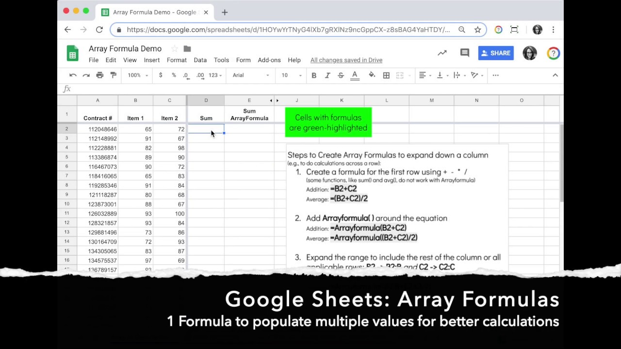
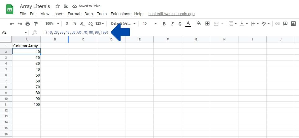
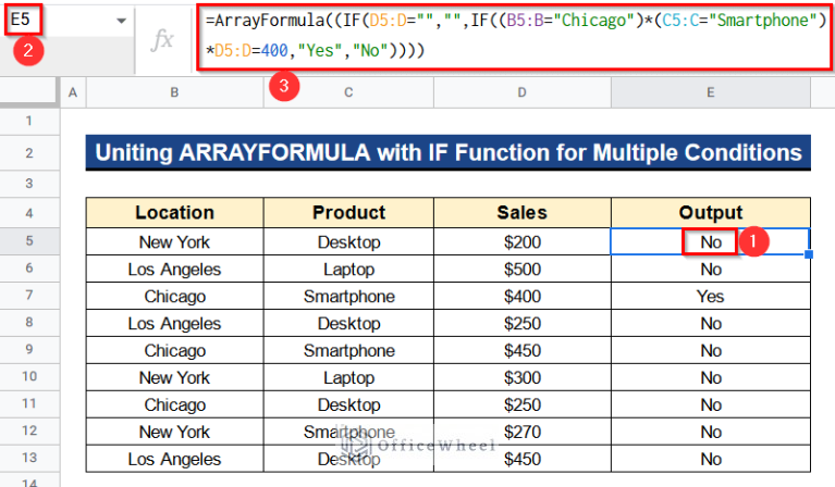
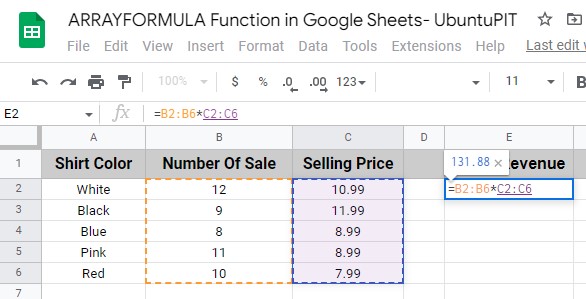
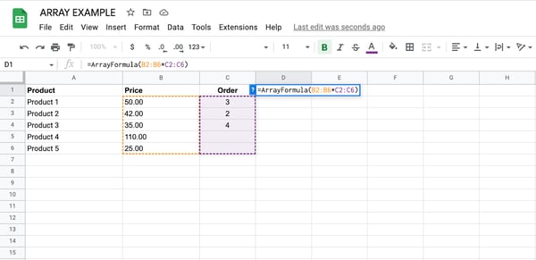
An array formula in Google Sheets is a powerful tool that allows you to perform multiple calculations on one or more items in a data set and return either a single result or a range of results. By using the ARRAYFORMULA function, you can apply a single formula to an entire column or row, eliminating the need to manually drag formulas down and ensuring that new data is automatically included in your calculations.
Understanding the Logic of Array Formulas
At its core, the array formula is about efficiency and scalability. In a traditional spreadsheet workflow, if you wanted to multiply the values in Column A by the values in Column B, you would write =A2*B2 in cell C2 and then "drag" that formula down to the bottom of your data set. While this works for small tables, it becomes a maintenance nightmare as your data grows. If you add 100 new rows, you must remember to drag the formula down again. If you accidentally change the formula in row 50, your data becomes inconsistent.
The ARRAYFORMULA function changes this paradigm by treating a range of cells as a single entity. Instead of calculating one cell at a time, Google Sheets processes the entire array in one go. In 2026, with the increased complexity of cloud-based data management, mastering this function is no longer just an "advanced tip"; it is a prerequisite for building robust, automated dashboards and financial models.
When you wrap a standard calculation in ARRAYFORMULA, you are telling Google Sheets: "Take this logic and repeat it for every row in the specified range." This results in what is often called "spilling," where the results flow out from the master cell into the cells below or to the right, depending on the dimensions of your input ranges.
Basic Syntax and the Ctrl+Shift+Enter Shortcut
The formal syntax for the function is:
=ARRAYFORMULA(array_formula)
The array_formula argument can be a mathematical operation, a range, or a combination of other functions that support array processing.
One of the most useful features for power users is the keyboard shortcut. While typing a formula, you can press Ctrl + Shift + Enter (Windows) or Cmd + Shift + Enter (Mac). Google Sheets will automatically wrap your current formula in the ARRAYFORMULA() wrapper. This is a significant time-saver and reduces the likelihood of syntax errors caused by missing parentheses.
Example: Simple Multiplication across a Column
If you have "Quantity" in A2:A100 and "Price" in B2:B100, you can calculate the "Total" in C2 with a single formula:
=ARRAYFORMULA(A2:A100 * B2:B100)
Instead of 99 individual formulas, you have one. If you change the logic in C2, the entire column updates instantly.
Handling Infinite Ranges with the A:A Syntax
One of the primary reasons professionals use array formulas in 2026 is to accommodate dynamic data entry, such as responses from a Google Form or live API data. By using "open-ended" ranges, you ensure your calculations never break as new rows are added.
Instead of defining a range like A2:A100, you can use A2:A. This tells Google Sheets to start at row 2 and continue until the very last row of the spreadsheet.
=ARRAYFORMULA(A2:A * B2:B)
However, using infinite ranges introduces a common aesthetic and functional problem: Google Sheets will attempt to calculate the formula for every single row, including thousands of empty rows at the bottom of your sheet. This can result in a column of zeros or error messages where no data exists.
The IF and LEN Trick: Preventing Calculation in Empty Rows
To maintain a clean spreadsheet, you must combine your array formula with logical checks. The most common method involves the IF and LEN functions. The goal is to tell the spreadsheet: "Only perform this calculation if there is actually data in the row."
The standard pattern is:
=ARRAYFORMULA(IF(LEN(A2:A), A2:A * B2:B, ""))
In this formula:
LEN(A2:A)checks the length of the content in Column A. If the cell is empty, the length is 0, which evaluates to "False" in a logical context.- If data exists, it performs the multiplication.
- If no data exists, it returns an empty string (
""), leaving the cell appearing blank.
Using IF(A2:A="",, ...) is another popular variation that achieves the same result by specifically looking for empty cells. This practice is essential for performance optimization in large-sized workbooks, as it prevents the calculation engine from processing unnecessary operations on thousands of null values.
Advanced Logic: Array Formulas with VLOOKUP
The VLOOKUP function is one of the most used tools in Google Sheets, but it is traditionally limited to looking up a single value. When paired with ARRAYFORMULA, it becomes a powerhouse capable of performing a "bulk lookup."
Suppose you have a list of Product IDs in Column A and a reference table on another tab. To pull the Product Name for every ID in Column A at once:
=ARRAYFORMULA(VLOOKUP(A2:A, 'Reference Tab'!A:B, 2, FALSE))
Here, the search key is not just A2, but the entire range A2:A. Google Sheets will return an array of names that corresponds to the IDs. This is significantly more efficient than copying a VLOOKUP down 10,000 rows, as it reduces the overhead on the Google Sheets calculation engine.
The Evolution: ARRAYFORMULA vs. Lambda Helper Functions
By 2026, the landscape of Google Sheets has matured to include "Lambda Helper Functions" (LHFs) such as MAP, BYROW, BYCOL, and SCAN. While ARRAYFORMULA remains the standard for basic arithmetic and simple logic, it has inherent limitations. Specifically, certain functions like SUM, AVERAGE, COUNT, and SUMIF do not work "inside" an ARRAYFORMULA when you want them to process row-by-row.
For example, if you try =ARRAYFORMULA(SUM(A2:B2)) and drag it down, it works. But if you try =ARRAYFORMULA(SUM(A2:B)) hoping to get a row-by-row sum, Google Sheets will instead sum the entire range and return a single value.
To solve this, we now use BYROW:
=BYROW(A2:B, LAMBDA(row, SUM(row)))
When to use which?
- Use
ARRAYFORMULAfor: Addition, subtraction, concatenation,VLOOKUP,IF, and basic comparisons. - Use
MAPorBYROWfor: Aggregation functions (SUM, COUNT), complex custom logic, or when you need to refer to a "current row" context thatARRAYFORMULAcannot provide.
Comparison Table: Formula Execution Methods
| Feature | Drag-and-Fill | ARRAYFORMULA | MAP / LAMBDA |
|---|---|---|---|
| Maintenance | High (manual updates) | Low (one formula) | Low (one formula) |
| Performance | Slower (many instances) | Fast (batch processing) | Moderate to Fast |
| Learning Curve | Beginner | Intermediate | Advanced |
| Best For | Ad-hoc, small tasks | Large datasets, simple math | Complex row-by-row logic |
| Infinite Ranges | No | Yes (A2:A) | Yes |
| Aggregation (SUM) | Yes (per cell) | No (collapses array) | Yes (using BYROW) |
Common Errors and Troubleshooting
The #REF! "Overwrite" Error
The most common error users encounter is the #REF! error with the message: "Array result was not expanded because it would overwrite data in [Cell].".
Because an array formula "spills" its results into the cells below it, those cells must be completely empty. If you have even a single space or a stray character in cell A10, and your array formula starts at A1 and needs to reach A20, the entire formula will fail. To fix this, simply clear the range where the formula is trying to expand.
The "Circular Dependency" Error
This happens if your array formula range includes the cell where the formula itself is located. For example, putting =ARRAYFORMULA(A1:A * 1.1) inside cell A1 will cause an infinite loop. Always ensure your formula is placed in a column or row outside the input range, or start the range from the row below the header (e.g., placing the formula in B2 and referencing A2:A).
Mismatched Range Sizes
For an array formula to work correctly across multiple columns, the ranges must be of equal size. =ARRAYFORMULA(A2:A10 + B2:B20) will result in an error or unexpected behavior because the two arrays have different lengths. Always ensure your ranges start and end at the same row numbers.
Performance Considerations for 2026
Google Sheets has seen significant backend optimizations by 2026, allowing it to handle hundreds of thousands of cells more gracefully than in previous decades. However, array formulas are not a magic bullet for speed.
A single ARRAYFORMULA is generally more efficient than 5,000 individual formulas because the spreadsheet only has to parse the syntax once. However, "volatile" functions—those that recalculate every time you make a change (like NOW(), RAND(), or INDIRECT())—can slow down your sheet significantly if wrapped in an array.
Furthermore, avoid nesting too many complex functions within a single ARRAYFORMULA. If you find yourself writing a formula that is ten lines long, it may be better to break it into "helper columns" or utilize Google Apps Script for more intensive data processing.
Practical Implementation: A Step-by-Step Workflow
To implement a professional-grade array formula, follow these steps:
- Prepare your Headers: Ensure your top row is frozen and labeled.
- Write the Base Formula: Start with the logic for a single row (e.g.,
=A2*B2). - Convert to Array: Add the range (e.g.,
=A2:A*B2:B) and press Ctrl+Shift+Enter. - Add Logic for Empty Rows: Wrap the formula in an
IF(LEN())statement to keep the bottom of your sheet clean. - Verify the Spillage: Delete any manual data in the output column to allow the formula to expand fully.
- Test with New Data: Add a new row of data at the bottom of your sheet to ensure the formula automatically calculates the result.
Frequently Asked Questions
Can I use ARRAYFORMULA with checkboxes?
Yes. If you have a column of checkboxes (True/False values), you can use an array formula to perform actions based on whether they are checked. For example, =ARRAYFORMULA(IF(A2:A=TRUE, "Task Completed", "Pending")) will instantly update the status for every checkbox in the column.
Why doesn't SUMIF work with ARRAYFORMULA?
SUMIF and COUNTIF are designed to take a range and return a single value. When you try to use them inside an ARRAYFORMULA to get a row-by-row total, they usually fail to iterate correctly. In these cases, you should use the SUMIFS function (which sometimes behaves better) or, preferably, the MAP function combined with SUM or SUMIF.
Is there a limit to how many rows an array formula can handle?
Google Sheets has a limit of 10 million cells per spreadsheet as of 2026. While an array formula can theoretically handle all those rows, performance will degrade as you approach the limit. If you are working with more than 100,000 rows of complex array calculations, consider using a database solution like BigQuery and connecting it to Sheets.
Can I use ARRAYFORMULA to combine text from different columns?
Absolutely. This is one of the most common uses. To combine First Name (A) and Last Name (B) with a space in between, use:
=ARRAYFORMULA(A2:A & " " & B2:B)
This is much more efficient than using the CONCATENATE function, which does not naturally support array expansion across rows.
How do I stop an array formula at a certain row?
If you don't want the formula to go to the very bottom of the sheet, simply define the end of the range. Instead of A2:A, use A2:A100. The formula will stop calculating at row 100, regardless of how much more data you add.
Recommendation for Next Actions
For users looking to streamline their spreadsheets in 2026, the first step is to audit existing workbooks for "formula drag." Identify columns where you are manually copying formulas and replace them with a single ARRAYFORMULA wrapped in an IF(LEN()) check.
Once you are comfortable with basic array logic, explore the Lambda Helper Functions (MAP, BYROW). These represent the next tier of spreadsheet automation and provide the flexibility needed for calculations that ARRAYFORMULA cannot handle. By transitioning to these array-based methods, you create spreadsheets that are not only faster but also significantly more resistant to manual entry errors.