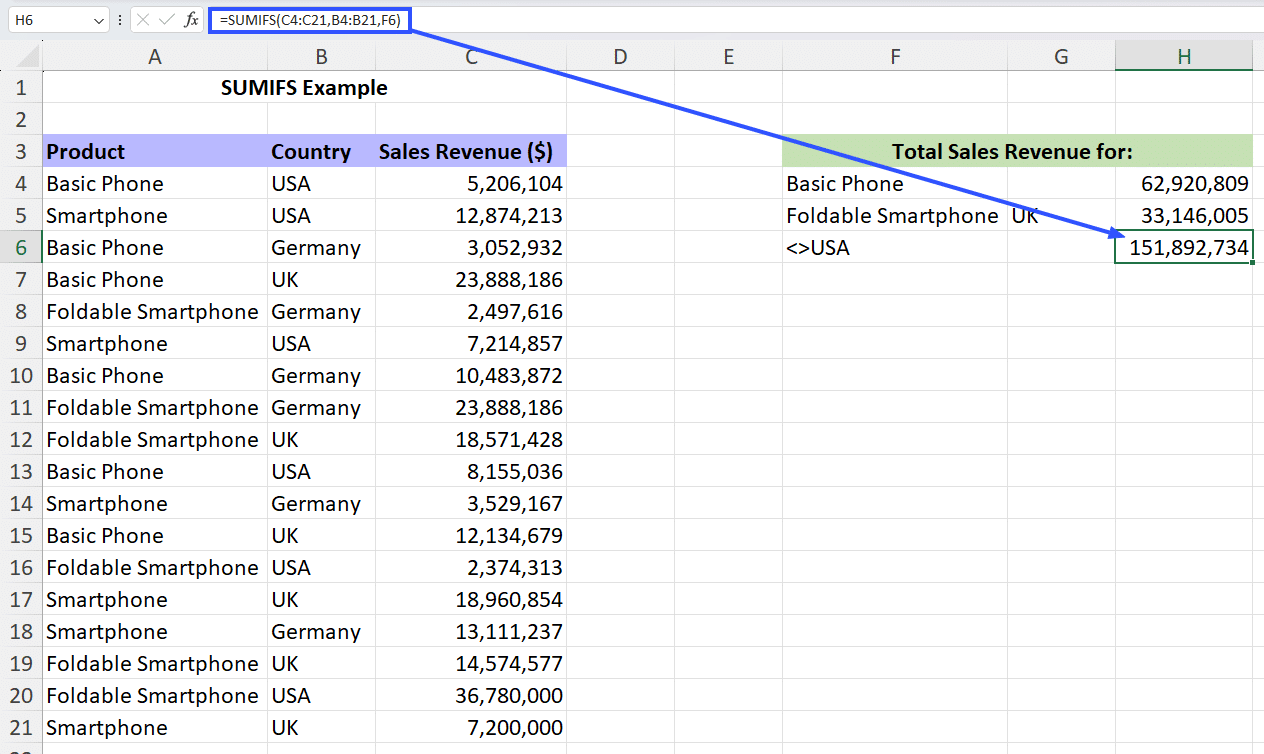
The SUMIFS function in spreadsheet applications like Microsoft Excel and Google Sheets calculates the sum of a range of cells when multiple conditions, or criteria, are met simultaneously. By structuring the formula as =SUMIFS(sum_range, criteria_range1, criteria1, criteria_range2, criteria2), users can filter datasets by two or more specific parameters to pull precise financial, operational, or analytical totals.
Introduction to Conditional Summation
Data analysis often requires looking past broad aggregates to examine how specific subsets perform. While a standard SUM function adds an entire column of numbers, and a SUMIF function evaluates a single condition, real-world data analysis almost always demands multidimensional evaluation. For instance, a sales manager may want to know not just total revenue, but the total revenue generated by a specific sales representative within a specific region. Similarly, an inventory manager might need to calculate the total stock value of items that belong to a specific category and are stored in a designated warehouse.
The SUMIFS formula addresses this exact operational requirement. Introduced to handle multiple criteria natively without cumbersome nested formulas or complex array syntax, SUMIFS acts as an advanced data-filtering and aggregation tool. Understanding how to construct a SUMIFS formula with two criteria transforms raw, unorganized rows of data into structured, actionable insights. Whether you are managing personal budgets, analyzing corporate expenditures, or tracking project milestones, mastering multi-criteria summation is an essential technical competency for modern spreadsheet users.
The Syntax and Logic Behind SUMIFS
Before building a two-criteria formula, it is vital to master the syntax and structural logic that spreadsheet applications require. Unlike its predecessor SUMIF, where the summation range is placed at the end of the argument list, SUMIFS places the summation range first. This architectural change allows the function to accept an indefinite number of criteria range and criteria pairs.
The standard syntax for a two-criteria SUMIFS formula is structured as follows:
=SUMIFS(sum_range, criteria_range1, criteria1, criteria_range2, criteria2)
Each component of this formula plays a distinct structural role:
sum_range: The actual range of cells that you want to add together. These must be numeric values; text or logical values within this range are ignored.criteria_range1: The first range of cells that will be evaluated against your first condition.criteria1: The condition that must be met withincriteria_range1. This can be a number, text string, cell reference, or logical expression (e.g.,">100","North", orA2).criteria_range2: The second range of cells that will be evaluated against your second condition.criteria2: The condition that must be met withincriteria_range2.
A critical rule to remember when building this formula is that range sizes must match. If sum_range spans from row 2 to row 100, then criteria_range1 and criteria_range2 must also span from row 2 to row 100. Mismatched range dimensions will result in a #VALUE! error or incorrect mathematical evaluations.
Preparing Your Data for Multi-Criteria Analysis
Even the most accurately constructed formula will fail or yield erroneous results if the underlying dataset is poorly structured. Spreadsheet applications rely on consistent data formatting to evaluate conditions accurately. Before applying a SUMIFS formula with two criteria, you must audit your dataset for common structural flaws.
Data Uniformity and Formatting
First, ensure that your data is organized in a tabular format, where each column represents a single category of information (e.g., Date, Region, Salesperson, Product, Revenue) and each row represents a single record.
- Text Consistency: Text criteria are case-insensitive in standard Excel and Google Sheets configurations, but they are highly sensitive to trailing spaces and typos. For example, the text string
"North "(with a trailing space) will not match"North", causing theSUMIFSfunction to skip that row entirely. - Numeric Integrity: Ensure that numbers in your
sum_rangeare stored as actual numeric values, not as text strings. Numbers formatted as text will be ignored by the summation engine, leading to understated totals. - Date Standardization: If one of your two criteria involves dates, ensure all dates within that criteria range use the exact same date serial format recognized by your spreadsheet application.
| Data Row | Column A (Region) | Column B (Product) | Column C (Revenue) | Status Check |
|---|---|---|---|---|
| Row 2 | North | Widgets | $1,200 | Valid Numeric Value |
| Row 3 | South | Gadgets | $850 | Valid Numeric Value |
| Row 4 | North | Widgets | $430 | Valid Numeric Value |
| Row 5 | East | Gizmos | $1,100 | Valid Numeric Value |
Step-by-Step Guide: Building a Two-Criteria SUMIFS Formula
To understand how this formula operates in a live environment, let us walk through a practical scenario. Imagine you manage a regional sales team. You have a dataset where Column A contains the Sales Region, Column B contains the Product Category, and Column C contains the total sales revenue. You want to calculate the total revenue generated specifically by the North region for the Widgets product category.
Step 1: Identify Your Ranges and Criteria
- Sum Range (Revenue):
C2:C100 - First Criteria Range (Region):
A2:A100 - First Criterion:
"North" - Second Criteria Range (Product):
B2:B100 - Second Criterion:
"Widgets"
Step 2: Enter the Formula Structure
Click on the cell where you want the final sum to appear. Type the equal sign to initiate the formula, followed by the function name and open parenthesis:
=SUMIFS(
Step 3: Add the Sum Range
Select or type the range containing the numeric values you want to sum. Type a comma to separate this argument from the next:
=SUMIFS(C2:C100,
Step 4: Add the First Criterion Pair
Incorporate your first criteria range and the specific condition you are evaluating. Enclose text criteria in quotation marks unless you are referencing a cell that contains the text:
=SUMIFS(C2:C100, A2:A100, "North",
Step 5: Add the Second Criterion Pair and Close
Incorporate your second criteria range and second condition, then close the parentheses to finalize the formula:
=SUMIFS(C2:C100, A2:A100, "North", B2:B100, "Widgets")
Press Enter, and the cell will instantly calculate the aggregate sum of all rows where Column A equals "North" and Column B equals "Widgets".
Using Cell References Instead of Hardcoded Text
While typing hardcoded text strings like "North" directly into a formula is useful for quick calculations, it limits the dynamic flexibility of your spreadsheet. Professional spreadsheet design relies on cell references, allowing users to change criteria dynamically without editing the formula string itself.
Instead of writing:
=SUMIFS(C2:C100, A2:A100, "North", B2:B100, "Widgets")
You can place your criteria in dedicated cells on your worksheet—for example, placing "North" in cell E1 and "Widgets" in cell E2. Your formula then becomes:
=SUMIFS(C2:C100, A2:A100, E1, B2:B100, E2)
This approach offers several operational advantages:
- Dashboard Creation: Users can build interactive dashboards where changing a drop-down menu in cell
E1instantly updates multipleSUMIFScalculations across the sheet. - Error Reduction: Minimizes the risk of typos occurring deep within complex formula strings during routine updates.
- Auditability: Makes the active criteria immediately visible to anyone reviewing the workbook.
Incorporating Logical Operators and Wildcards
The true power of the SUMIFS formula emerges when you move beyond exact matches and incorporate logical operators and wildcard characters into your criteria arguments.
Using Logical Operators
When evaluating numerical ranges or dates with your two criteria, you can combine comparison operators with your criteria strings. Operators must be enclosed in quotation marks and joined to cell references or numbers using an ampersand (&).
For example, to calculate total sales for the North region where sales revenue is greater than 500, the formula would look like this:
=SUMIFS(C2:C100, A2:A100, "North", C2:C100, ">500")
If your threshold value is stored in cell E3, the syntax requires an ampersand concatenation:
=SUMIFS(C2:C100, A2:A100, "North", C2:C100, ">"&E3)
Using Wildcards for Partial Matches
When dealing with text criteria, you can use wildcard characters to match partial strings:
- Asterisk (
*): Represents any sequence of characters. For example,"*Widget*"will match any product description containing the word "Widget," regardless of what precedes or follows it. - Question Mark (
?): Represents any single character. For example,"Bx"will match "Box", "Bax", or "Bix".
For instance, if your first criterion is the North region and your second criterion is any product starting with "Smart", your formula would be:
=SUMIFS(C2:C100, A2:A100, "North", B2:B100, "Smart*")
Common Mistakes and Troubleshooting
Even experienced spreadsheet users occasionally encounter errors when building multi-criteria formulas. Understanding common pitfalls helps diagnose and resolve issues quickly.
1. The Mismatched Range Dimensions Error (#VALUE!)
- The Cause: Your
sum_rangeand your criteria ranges do not share the exact same number of rows or columns. For example, ifsum_rangeisC2:C100(99 rows) whilecriteria_range1isA2:A50(49 rows), the application cannot align the datasets. - The Fix: Ensure all ranges in the formula argument list reference identically sized arrays (e.g.,
C2:C100,A2:A100, andB2:B100).
2. Missing Quotation Marks on Logical Operators
- The Cause: Writing mathematical conditions without enclosing the operator in quotation marks (e.g., writing
>500instead of">500"). Spreadsheet applications will evaluate this as a syntax error. - The Fix: Always enclose operators and text strings in double quotation marks.
3. Text Formatting and Invisible Spaces
- The Cause: Data imported from external databases often contains trailing or leading whitespace characters that prevent exact-match criteria from evaluating properly.
- The Fix: Clean your source data using the
TRIMfunction in a helper column before running yourSUMIFSanalysis, or audit your criteria cell for accidental spaces.
Frequently Asked Questions
Can SUMIFS handle more than two criteria?
Yes. While this guide focuses on two criteria, the SUMIFS function can evaluate up to 127 individual criteria range and criteria pairs in modern versions of Microsoft Excel and Google Sheets. Simply append additional range and condition pairs to the end of the formula string following the established syntax pattern.
Are SUMIFS criteria case-sensitive?
No. By default, standard text criteria in SUMIFS are case-insensitive. Searching for "north" will return the exact same mathematical result as searching for "NORTH" or "North". If you require strict case-sensitive summation, you must combine SUMPRODUCT with exact-matching functions like EXACT.
What happens if no rows match my two criteria?
If none of the rows in your dataset satisfy all specified criteria simultaneously, the SUMIFS formula will return 0. It does not return an error code when zero matches are found, which makes checking your criteria logic essential if you expected a positive value.
Can I use OR logic instead of AND logic in SUMIFS?
By design, SUMIFS operates strictly on AND logic—meaning every single condition must be met for a row to be included in the sum. To evaluate OR logic across multiple criteria (e.g., summing items that are either in the North region OR the South region), you can add multiple SUMIFS formulas together, such as =SUMIFS(C2:C100, A2:A100, "North") + SUMIFS(C2:C100, A2:A100, "South").
Why is my formula returning zero even though the data looks correct?
The most common reasons for a zero result are numeric values formatted improperly as text strings within the sum_range, or mismatched criteria spelling between your formula string and your data table. Check that your numbers are right-aligned (indicating numeric storage) and that text strings match character-for-character.
Summary and Next Actions
Mastering the SUMIFS formula with two criteria unlocks advanced reporting capabilities in spreadsheet applications. By establishing proper tabular data formatting, arranging your syntax with the sum range first, and leveraging cell references or logical operators, you can automate complex data aggregation tasks.
To reinforce your learning:
- Open a practice spreadsheet containing a clean table of sales, inventory, or financial data.
- Construct a baseline
SUMIFSformula using two distinct text criteria. - Replace hardcoded text strings with cell references to test dynamic dashboard updates.
- Experiment with logical operators like
">"or wildcard characters like"*"to refine your analytical filtering.