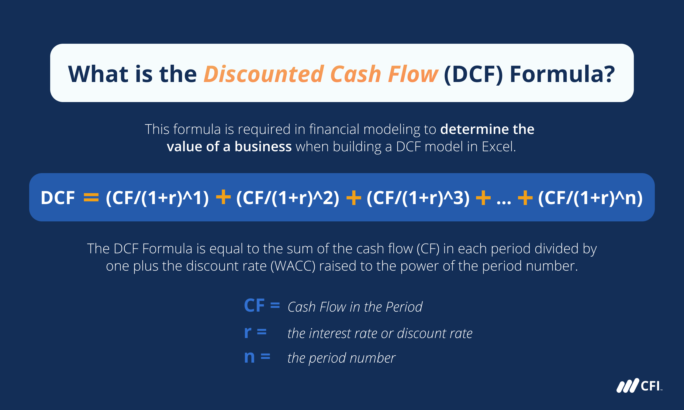
A discounted cash flow (DCF) analysis determines the intrinsic value of an investment by forecasting its future cash flows and discounting them back to their present value using a specific discount rate. This method allows investors to assess whether an asset is overvalued or undervalued based on its ability to generate cash in the future.
The discounted cash flow model remains the gold standard of fundamental valuation in 2026. While market sentiment and multiples-based valuation (like P/E ratios) offer a snapshot of current demand, the DCF analysis peers into the actual economic engine of a business. It rests on the principle of the "Time Value of Money"—the concept that a dollar today is worth more than a dollar tomorrow because today's dollar can be invested to earn interest. To perform a robust DCF, an analyst must combine historical data with forward-looking assumptions, balancing mathematical precision with professional judgment.
Step 1: Forecast the Financial Statements and Free Cash Flow
The foundation of any DCF analysis is a reliable forecast. Before you can discount cash flows, you must estimate what those flows will be. Most analysts use a five-to-ten-year projection period, depending on the maturity of the business. For a stable company, five years is often sufficient; for a high-growth startup, ten years may be necessary to reach a "steady state."
The primary metric used is Unlevered Free Cash Flow (UFCF). Unlike net income, which includes non-cash accounting entries, UFCF represents the actual cash available to all capital providers (both debt and equity holders). To calculate UFCF, start with Earnings Before Interest and Taxes (EBIT). Subtract the estimated taxes to reach the Net Operating Profit After Taxes (NOPAT). From there, add back non-cash expenses like Depreciation and Amortization (D&A), subtract Capital Expenditures (CapEx), and adjust for changes in Net Working Capital (NWC).
This step requires a deep dive into the company’s revenue drivers. You must consider market share, pricing power, and volume growth. A common mistake is assuming constant growth without considering the competitive landscape or capital intensity required to sustain that growth.
Step 2: Determine the Forecast Period Length
Choosing the right time horizon is a strategic decision. If the forecast period is too short, you might miss the long-term value creation of a growing firm. If it is too long, the projections become speculative and unreliable. In 2026, many analysts favor a two-stage DCF model: a high-growth stage followed by a transition to a stable terminal growth stage.
During the forecast period, you should reflect "mean reversion." If a company is currently earning extraordinary margins, competition will likely compress those margins over time. Your year-by-year projections should show the company gradually reaching a "normalized" state of operations. This normalization includes aligning Capital Expenditures with Depreciation—suggesting the company is investing just enough to maintain its assets rather than aggressively expanding.
Step 3: Calculate the Change in Net Working Capital
Net Working Capital (NWC) is often the most overlooked component of a DCF. It represents the liquidity required to run day-to-day operations. It is calculated as Current Assets (excluding cash) minus Current Liabilities (excluding debt). As a company grows, it typically needs more inventory and carries more accounts receivable, which "traps" cash.
When calculating the change in NWC for your DCF, an increase in working capital is a cash outflow, while a decrease is a cash inflow. For example, if a company speeds up its collections from customers (reducing Accounts Receivable), its cash flow improves. Conversely, if it must stockpile inventory to meet 2026 supply chain demands, that cash is no longer available to investors. Accuracy here requires analyzing historical ratios, such as Days Sales Outstanding (DSO) and Inventory Turnover.
Step 4: Estimate the Terminal Value
Since a business is theoretically an "ongoing concern" that exists forever, you cannot project cash flows to infinity. Instead, you project for a set period and then calculate a Terminal Value (TV) to represent the value of all cash flows beyond that period. Terminal Value often accounts for 60% to 80% of the total DCF result, making it a highly sensitive variable.
There are two primary methods to calculate Terminal Value:
- Perpetuity Growth Method (Gordon Growth Model): This assumes the company will grow its cash flows at a constant, modest rate forever. This rate is usually pegged to the long-term inflation rate or the GDP growth rate (typically 2% to 3%).
- Exit Multiple Method: This assumes the business is sold at the end of the forecast period for a multiple of its EBITDA (Earnings Before Interest, Taxes, Depreciation, and Amortization). This multiple is derived from comparable companies currently trading in the market.
Using both methods and averaging the results—or using one to "sanity check" the other—is a best practice for modern financial modeling.
Step 5: Determine the Discount Rate (WACC)
The discount rate reflects the risk of the investment and the opportunity cost of capital. For an unlevered DCF, the appropriate rate is the Weighted Average Cost of Capital (WACC). WACC blends the cost of equity and the after-tax cost of debt based on the company’s capital structure.
To find the Cost of Equity, most analysts use the Capital Asset Pricing Model (CAPM). This formula is: Cost of Equity = Risk-Free Rate + (Beta × Equity Risk Premium)
In 2026, the risk-free rate is typically derived from the yield on 10-year government bonds. Beta measures the stock's volatility relative to the market, and the Equity Risk Premium represents the extra return investors demand for holding stocks over "risk-free" bonds. The Cost of Debt is easier to find; it is the effective interest rate the company pays on its borrowings, adjusted for the tax shield (since interest is tax-deductible).
Step 6: Discount the Cash Flows to Present Value
Once you have your annual Free Cash Flows, the Terminal Value, and the WACC, you must "bring them back" to today's dollars. This is done using the PV formula: PV = CF / (1 + r)^n
Where CF is the cash flow in a given year, r is the discount rate (WACC), and n is the year number. For the Terminal Value, you discount it back by the total number of years in your forecast period.
Many professionals use the Mid-Year Convention for higher accuracy. This assumes that cash flows are received evenly throughout the year rather than in one lump sum on December 31st. This is achieved by using (n - 0.5) as the exponent in the discounting formula. This small adjustment can significantly impact the valuation, especially for companies with large annual cash flows.
Step 7: Calculate the Enterprise Value
The Enterprise Value (EV) is the sum of the present values of all projected free cash flows plus the present value of the Terminal Value. This figure represents the total value of the firm's core business operations. It is the price an acquirer would pay to buy the entire business, assuming they take over all debt and keep all cash.
At this stage, it is crucial to ensure that the units are consistent. If your projections are in millions, your final EV must be as well. The Enterprise Value is a "capital neutral" figure, meaning it is the value of the assets regardless of how those assets were financed (debt vs. equity).
Step 8: Adjust for Net Debt and Non-Operating Items
To find the value specifically attributable to shareholders, you must move from Enterprise Value to Equity Value. This is done by subtracting any claims that take priority over common shareholders and adding back assets that were not included in the Free Cash Flow projections.
The standard bridge is:
- Subtract Total Debt: Short-term and long-term loans, bonds, and notes payable.
- Add Cash and Cash Equivalents: This is "excess" cash that can be used to pay off debt or distributed to shareholders.
- Subtract Minority Interest: If the company consolidated a subsidiary it doesn't fully own, the portion it doesn't own must be subtracted.
- Subtract Preferred Stock: These shareholders are higher in the "capital stack" than common stockholders.
This result is the Equity Value, often referred to as the "Market Cap" if the company were priced perfectly by the market.
Step 9: Calculate the Intrinsic Value per Share
For individual investors, the final goal is usually to determine if a single share of stock is a good deal. To do this, divide the total Equity Value by the fully diluted shares outstanding.
It is important to use the diluted count rather than the basic count. Diluted shares include not just the shares currently trading, but also potential shares from "in-the-money" stock options, warrants, and convertible bonds. In 2026, stock-based compensation remains a significant expense for tech and growth companies, making dilution a critical factor in valuation. If your calculated intrinsic value is $150 and the stock is currently trading at $120, the DCF suggests the stock is undervalued by 20%.
Step 10: Perform Sensitivity Analysis
A DCF is only as good as its inputs. Because small changes in the WACC or the terminal growth rate can cause massive swings in the final share price, a Sensitivity Analysis (often called a "what-if" analysis) is mandatory.
Create a "Sensitivity Table" (often a data table in Excel) that shows the share price at various combinations of WACC and Terminal Growth Rates. This allows you to see the "Margin of Safety." If the stock is undervalued only if the company grows at 5% forever, but it's overvalued if it grows at 2%, the investment is risky. A robust investment thesis usually requires the stock to be undervalued even under conservative or "bear case" assumptions.
Comparison of Terminal Value Methods
| Feature | Perpetuity Growth Method | Exit Multiple Method |
|---|---|---|
| Core Assumption | Business grows at a constant rate forever. | Business is sold based on market benchmarks. |
| Best Used For | Mature companies in stable industries. | High-growth industries or private equity exits. |
| Common Inputs | Long-term GDP growth, inflation, WACC. | LTM EBITDA, Industry-average EV/EBITDA. |
| Primary Risk | High sensitivity to the growth rate (g). | Subject to market "noise" and cycles. |
| Standard Benchmarks | Usually 1.5% to 3.0% growth. | Usually 8x to 15x EBITDA multiples. |
Frequently Asked Questions
What is the most sensitive variable in a DCF analysis? The discount rate (WACC) and the Terminal Growth Rate are the most sensitive. Because these numbers affect the "tail" of the valuation (the Terminal Value), a 1% change in WACC can often change the final valuation by 10% to 20%. This is why sensitivity analysis is a critical final step to understand the range of possible values.
Can I use DCF for a company with negative cash flows? Yes, but it is much more difficult. If a company is currently burning cash, you must forecast the exact point in the future when it becomes "cash flow positive." A DCF for a pre-revenue or high-burn company relies heavily on the "Stage 2" transition and requires very optimistic assumptions about reaching profitability, which increases the risk of the analysis.
How does a DCF differ from a Precedent Transactions analysis? A DCF is an "intrinsic" valuation based on the company's specific financials and future potential. A Precedent Transactions analysis is a "relative" valuation based on what other people have paid for similar companies in the past. While DCF tells you what a company should be worth based on cash, Precedent Transactions tell you what the market is actually willing to pay.
Is the DCF model still relevant in 2026? Absolutely. While AI-driven quantitative trading and high-frequency algorithms dominate daily price movements, the long-term price of an asset eventually converges with its ability to produce cash. In the volatile economic environment of 2026, the DCF provides a "North Star" for fundamental investors to avoid overpaying for speculative growth.
What is a "Margin of Safety" in DCF? The Margin of Safety is the difference between your calculated intrinsic value and the current market price. For example, if you calculate a value of $100 but the stock is trading at $70, you have a 30% margin of safety. This buffer protects you against errors in your forecasts or unexpected economic downturns.
Practical Recommendation for Next Actions
After completing your initial DCF, do not take the final number as an absolute truth. Instead, compare your results with a Comparable Company Analysis (Comps). If your DCF suggests the company is worth 25x EBITDA but all its competitors are trading at 10x EBITDA, your assumptions (likely your growth rate or WACC) may be too aggressive. Use the DCF as a tool to understand the drivers of value—ask yourself: "What would have to be true for this company to be worth this price?" This shift from "price-guessing" to "logic-testing" is the hallmark of a sophisticated analyst.