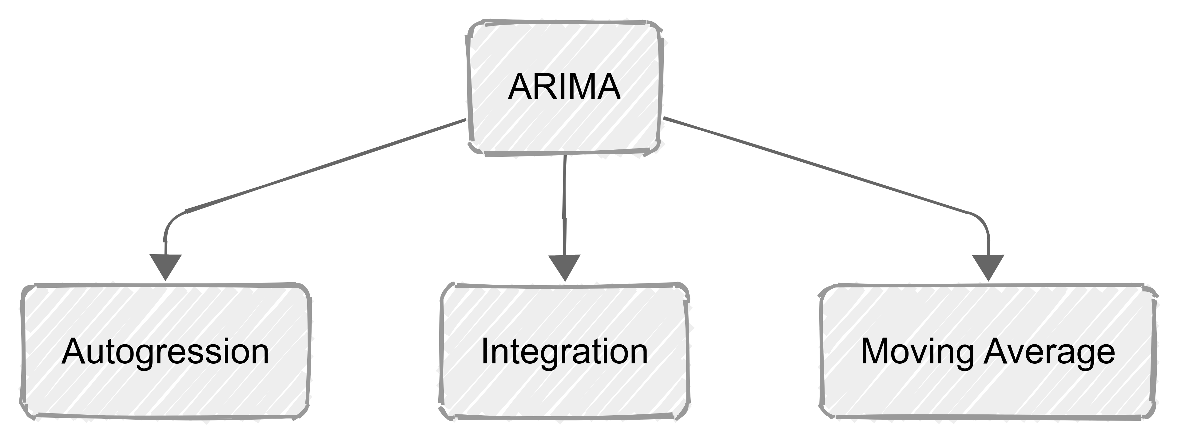
ARMA (Autoregressive Moving Average) and ARIMA (Autoregressive Integrated Moving Average) are foundational statistical models used to analyze and forecast time series data. ARMA is suitable for stationary data, combining past values and past errors, while ARIMA extends this by incorporating differencing (the "Integrated" component) to handle non-stationary data with trends.
Time series analysis remains a cornerstone of predictive analytics in 2026, bridging the gap between classical statistics and modern machine learning. Whether you are forecasting financial markets, energy consumption, or supply chain demand, understanding the mechanics of ARMA and ARIMA is essential for building robust, interpretable models. This guide explores the theoretical underpinnings, practical applications, and the critical differences between these two modeling powerhouses.
The Foundations of Time Series Modeling
To appreciate ARMA and ARIMA, one must first understand the unique nature of time series data. Unlike standard cross-sectional data, where observations are independent, time series data is sequential. The value of a variable today is often highly correlated with its value yesterday. This property, known as autocorrelation, is what these models seek to exploit.
The primary goal of these models is to describe the stochastic process of a variable over time. By identifying patterns in the data’s past—specifically its own previous values and the errors made in previous predictions—we can project those patterns into the future. In the context of 2026, where high-frequency data is ubiquitous, these models provide a computationally efficient way to generate forecasts without the "black box" complexity of deep learning.
The Concept of Stationarity
The most critical prerequisite for ARMA modeling is stationarity. A time series is stationary if its statistical properties, such as mean, variance, and autocorrelation, do not change over time. If a series has a clear upward trend or seasonal fluctuations that grow in magnitude, it is non-stationary.
Statisticians use tests like the Augmented Dickey-Fuller (ADF) test or the KPSS (Kwiatkowski-Phillips-Schmidt-Shin) test to verify stationarity. If a series is not stationary, it must be transformed—usually through differencing—before an ARMA model can be applied. This transformation process is precisely what leads us to the ARIMA model.
Breaking Down the ARMA Model (p, q)
The ARMA model is a combination of two distinct components: the Autoregressive (AR) part and the Moving Average (MA) part. It is typically denoted as ARMA(p, q), where 'p' is the order of the AR term and 'q' is the order of the MA term.
The Autoregressive (AR) Component
The AR part of the model suggests that the current value of the series is a linear combination of its own previous values plus an error term. The parameter 'p' represents the number of lagged observations included. For instance, an AR(1) model uses only the immediately preceding value to predict the current one.
In mathematical terms, an AR(p) model looks like this: Yt = c + φ1Yt-1 + φ2Yt-2 + ... + φpYt-p + εt
Here, Yt is the value at time t, c is a constant, φ represents the coefficients, and εt is white noise. The AR component is effective at capturing persistent trends or momentum in the data.
The Moving Average (MA) Component
The MA part of the model is often misunderstood. It does not refer to a simple moving average of the data points. Instead, it suggests that the current value is a linear combination of the current and past forecast errors (residuals). The parameter 'q' represents the number of lagged forecast errors.
The MA(q) model is expressed as: Yt = μ + εt + θ1εt-1 + θ2εt-2 + ... + θqεt-q
In this equation, μ is the mean of the series and θ represents the coefficients for the error terms. The MA component is particularly useful for capturing short-term shocks that dissipate over time, such as a sudden market correction or a temporary supply disruption.
Combining AR and MA
When we combine these two, we get the ARMA(p, q) model. This model assumes that the data is the result of both its past values and the shocks it has experienced. This dual approach makes ARMA highly flexible for modeling a wide variety of stationary time series.
The Role of Integration in ARIMA (p, d, q)
In the real world, very few time series are naturally stationary. Most economic, social, and physical data sets exhibit trends. This is where the ARIMA model becomes necessary. ARIMA stands for Autoregressive Integrated Moving Average.
The "I" stands for Integrated, which represents the differencing step required to make the data stationary. The ARIMA model is denoted as ARIMA(p, d, q), where 'd' is the degree of differencing.
Understanding Differencing (d)
Differencing involves subtracting the previous observation from the current observation: Y't = Yt - Yt-1
If a first-order difference (d=1) does not achieve stationarity, a second-order difference (d=2) can be applied, which is the difference of the differences. In practice, 'd' rarely exceeds 2. Differencing effectively removes the trend from the data, allowing the AR and MA components to focus on the underlying patterns of the stationary residuals.
The integration of differencing directly into the model framework (ARIMA) allows analysts to handle non-stationary data seamlessly. Once the forecast is made on the differenced data, the model automatically "re-integrates" or reverses the differencing to provide the forecast in the original scale of the data.
The Box-Jenkins Methodology
The standard approach to building an ARIMA model is known as the Box-Jenkins methodology. This systematic process ensures that the model is both accurate and parsimonious (using the fewest parameters possible).
1. Identification
The first step is to determine if the series is stationary. If it is not, the analyst determines the value of 'd' through differencing. Once stationarity is achieved, the Autocorrelation Function (ACF) and Partial Autocorrelation Function (PACF) plots are examined.
- ACF plots help identify the order of the MA term (q).
- PACF plots help identify the order of the AR term (p).
For example, if the PACF shows a sharp cutoff after two lags and the ACF decays slowly, it suggests an AR(2) process.
2. Estimation
Once p, d, and q are identified, the coefficients (φ and θ) are estimated. In 2026, this is almost exclusively done using maximum likelihood estimation (MLE) or least squares optimization via statistical software. The goal is to find the coefficients that minimize the errors between the model's predictions and the actual historical data.
3. Diagnostic Checking
After the model is built, it must be validated. The primary tool for this is residual analysis. If the model is a good fit, the residuals (the differences between predicted and actual values) should be white noise. This means they should have no discernible pattern, a mean of zero, and constant variance. The Ljung-Box test is commonly used to statistically verify that the residuals are independent.
4. Forecasting
Only after the model passes diagnostic checks is it used for forecasting. ARIMA models excel at short-to-medium-term forecasting. Because they rely on past values and errors, their accuracy generally decreases as the forecast horizon extends further into the future.
Comparative Analysis: ARMA vs. ARIMA
To choose the right model, one must understand their specific use cases and limitations.
| Feature | ARMA(p, q) | ARIMA(p, d, q) |
|---|---|---|
| Data Requirement | Strictly Stationary | Non-Stationary (with trend) |
| Key Components | AR + MA | AR + I + MA |
| Trend Handling | Cannot handle trends | Removes trends via differencing |
| Parameters | p (AR lags), q (MA lags) | p, d (differencing), q |
| Common Use Case | Highly controlled physical systems | Finance, Economics, Sales |
| Complexity | Lower | Moderate |
For more detailed information on time series specifications, the NIST Engineering Statistics Handbook provides comprehensive technical definitions and examples.
Advanced Variations and Extensions
In modern 2026 workflows, basic ARMA and ARIMA models are often the starting point for more complex variations:
- SARIMA (Seasonal ARIMA): Adds seasonal components to the model, denoted as (P, D, Q)s. This is essential for data with yearly, monthly, or weekly cycles, such as retail sales or weather patterns.
- ARIMAX: The "X" stands for exogenous variables. This allows the model to include external factors. For example, if you are forecasting electricity demand, an ARIMAX model could include temperature as an external regressor.
- GARCH (Generalized Autoregressive Conditional Heteroskedasticity): Often paired with ARIMA in finance, GARCH models the variance (volatility) of the errors, which is crucial for risk management.
For those interested in the rigorous mathematical proofs and latest developments in these extensions, the Journal of Time Series Analysis remains a primary source for peer-reviewed research.
Practical Challenges and Best Practices
While ARMA and ARIMA are powerful, they are not infallible. One of the most common mistakes is overfitting. Including too many lags (p or q) may make the model fit the historical noise perfectly but fail miserably when applied to new data. Using criteria like the Akaike Information Criterion (AIC) or Bayesian Information Criterion (BIC) helps in selecting a model that balances goodness-of-fit with simplicity.
Another challenge is the assumption of linearity. ARIMA is a linear model. If the underlying data-generating process is non-linear (e.g., chaotic systems or certain biological processes), ARIMA may provide suboptimal results. In such cases, hybrid models that combine ARIMA with machine learning techniques like Random Forests or LSTMs (Long Short-Term Memory networks) are often employed.
Finally, data quality is paramount. Outliers, missing values, and structural breaks (sudden changes in the underlying trend, such as a policy shift or a natural disaster) can lead to misleading ARIMA parameters. Pre-processing the data to handle these anomalies is a non-negotiable step in the modeling pipeline.
The Relevance of ARIMA in 2026
With the rise of sophisticated AI, some might ask if ARMA and ARIMA are still relevant in 2026. The answer is a resounding yes. These models offer interpretability that neural networks often lack. In regulated industries like banking and healthcare, being able to explain why a forecast was made is just as important as the forecast itself.
Furthermore, ARIMA models require significantly less data and computational power than deep learning models. For many business applications, the marginal gain in accuracy from a complex transformer model does not justify the increased cost and loss of transparency, making ARIMA the "Goldilocks" solution for many practitioners.
To see these models applied to real-world datasets, the Federal Reserve Economic Data (FRED) offers a wealth of time series data that serves as a perfect testing ground for ARIMA modeling.
Frequently Asked Questions
What is the difference between ARMA and ARIMA?
The primary difference is the "Integrated" (I) component. ARMA is designed for stationary data where the mean and variance are constant over time. ARIMA is designed for non-stationary data; it uses differencing to remove trends and stabilize the mean before applying the AR and MA components.
How do I choose the values for p, d, and q?
The value of 'd' is determined by how many times you must difference the data to make it stationary. The values of 'p' and 'q' are typically identified by looking at PACF and ACF plots, respectively. Additionally, automated model selection algorithms use the Akaike Information Criterion (AIC) to find the optimal combination of parameters.
Can ARIMA be used for long-term forecasting?
ARIMA is generally best suited for short-term to medium-term forecasting. Because the model relies on correlations with recent past values, its predictive power diminishes as you move further away from the last known data point. For very long-term structural changes, econometric models or causal models may be more appropriate.
What should I do if my data has seasonality?
If your data shows periodic patterns (like higher sales every December), a standard ARIMA model will fail to capture this. You should use a SARIMA (Seasonal ARIMA) model, which includes additional seasonal lags for the AR, MA, and Integrated components.
Is stationarity always required for ARIMA?
Technically, the "I" in ARIMA handles the non-stationarity. However, the data must be "integrable" to a stationary state. If the variance of the series increases over time (heteroskedasticity), you might need to apply a log transformation or a Box-Cox transformation before differencing.
Practical Recommendation
When starting a time series project, always begin with a visual inspection of your data. Plot the time series to look for trends, seasonality, and outliers. Perform an Augmented Dickey-Fuller test to check for stationarity. If the data is non-stationary, start with an ARIMA(0, 1, 0)—a simple random walk—and gradually add AR or MA terms based on the ACF and PACF plots. Always prioritize the simplest model that passes diagnostic tests (white noise residuals). This principle of parsimony will ensure your model is robust and generalizable to future data.