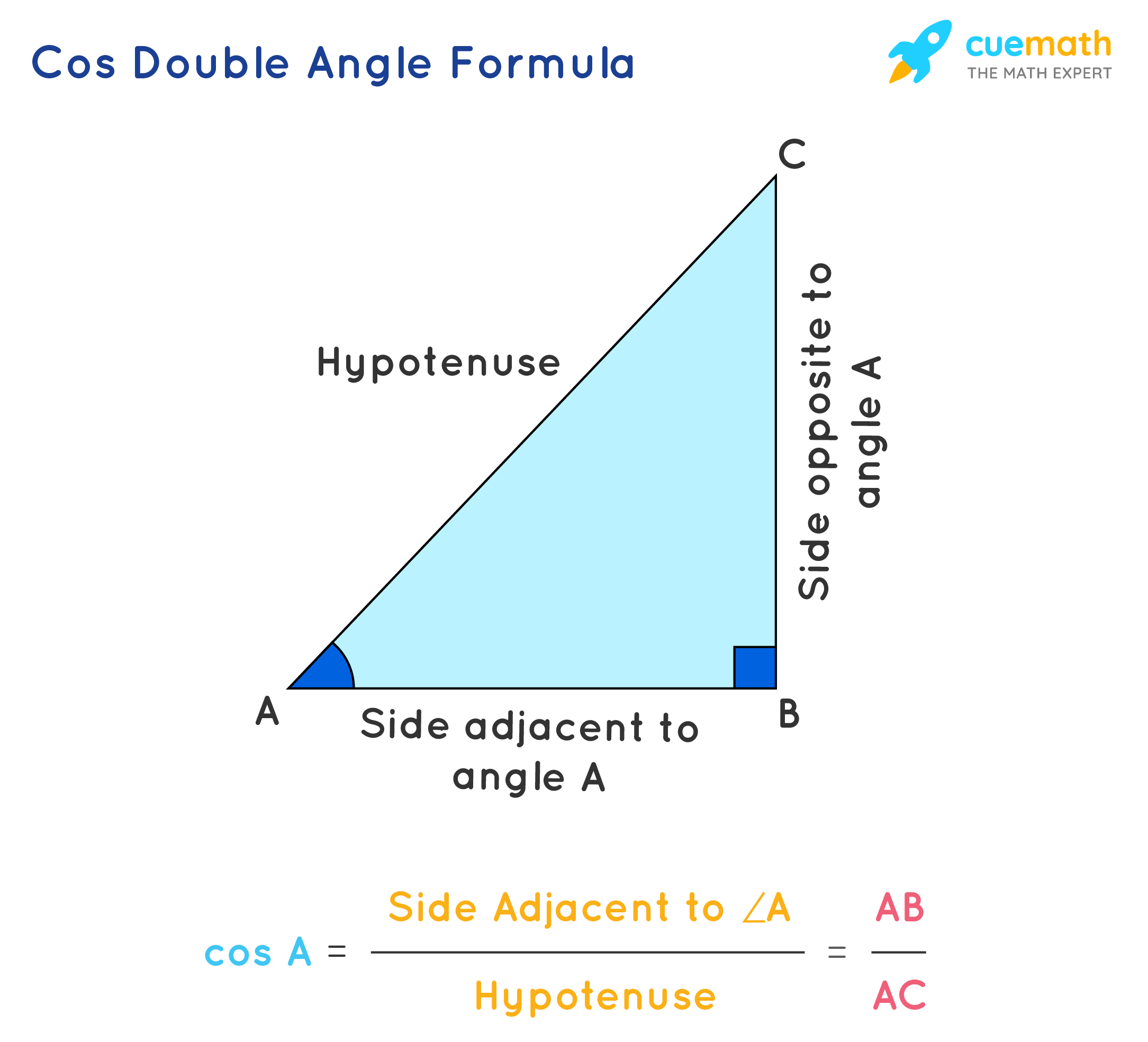
Trigonometric angle formulas—including basic right-triangle ratios, the Law of Cosines, the Law of Sines, and vector dot-product relations—translate raw spatial measurements into actionable geographic, structural, and computational data. In fields like land surveying, structural engineering, satellite navigation, game development, and physics, these formulas allow professionals to calculate unmeasurable distances, determine structural load distribution, program dynamic camera angles, and steer autonomous systems accurately.
Essential Trigonometric Angle Formulas at a Glance
In theoretical mathematics, trigonometric identities are often treated as abstract algebraic equations. In practical application, however, each formula serves as a specific computational tool tailored to the geometry of the problem and the available input data.
The table below outlines the primary angle formulas used across engineering, software development, and spatial science.
| Formula Name | Mathematical Expression | Required Inputs | Primary Practical Applications |
|---|---|---|---|
| Tangent Angle Formula | $\tan(\theta) = \frac{\text{Opposite}}{\text{Adjacent}}$ | One side length, one adjacent side, $90^\circ$ angle | Measuring tree/building heights, slope grading, optical elevation. |
| Law of Cosines (Angle Form) | $\cos(C) = \frac{a^2 + b^2 - c^2}{2ab}$ | All three side lengths ($a, b, c$) of any triangle | Obstacle clearance, navigation between three coordinates, 3D mesh modeling. |
| Law of Sines | $\frac{a}{\sin(A)} = \frac{b}{\sin(B)} = \frac{c}{\sin(C)}$ | Two angles and one side, or two sides and one non-included angle | Triangulation in geodesy, radio direction finding, astronomical parallax. |
| Vector Angle Formula | $\cos(\theta) = \frac{\mathbf{u} \cdot \mathbf{v}}{|\mathbf{u}| |\mathbf{v}|}$ | Coordinates of two 2D/3D vectors ($\mathbf{u}, \mathbf{v}$) | Game engine field-of-view (FOV), shading/lighting calculations, robotics path planning. |
| Two-Argument Arctangent | $\theta = \text{atan2}(y, x)$ | Planar coordinates $(x, y)$ | Computer graphics rotation, joystick input processing, autonomous vehicle steering. |
| Angle Addition Formula | $\sin(\alpha \pm \beta) = \sin\alpha\cos\beta \pm \cos\alpha\sin\beta$ | Two individual sub-angles ($\alpha, \beta$) | Signal processing phase shifts, 2D coordinate matrix rotation, acoustic wave analysis. |
Right-Triangle Trigonometry in Everyday Fieldwork
Right-triangle trigonometry forms the baseline of applied spatial measurement. When an observer can establish or assume a 90-degree angle relative to a baseline—such as gravity establishing a vertical line relative to a level ground plane—the classic ratios of sine, cosine, and tangent simplify complex physical measurements.
- Target Top
- Height (Opposite) vertical distance to Target Base
- Line $h$ (hypotenuse) to Observer
- Target Base
- Distance $d$ (Adjacent) horizontal distance to Observer
- Observer
- Angle $\theta$ between baseline (Distance $d$) and hypotenuse ($h$)
Measuring Height and Incline via Tangent Ratios
One of the most common applications of right-triangle trigonometry is indirect measurement using a clinometer or transit level. When measuring the height of an object (such as a telecommunications tower or tree canopy) where direct vertical measurement is impossible, field technicians use the tangent relationship:
$$\tan(\theta) = \frac{\text{Height}}{\text{Distance}}$$
Rearranging the formula yields:
$$\text{Height} = \text{Distance} \times \tan(\theta)$$
Worked Field Example:
A technician stands 45.0 meters away from the base of a utility tower on flat ground. Using a calibrated optical clinometer held at an eye level of 1.6 meters, the technician measures the angle of elevation to the top of the tower as $38.5^\circ$.
Calculate the vertical height above eye level: $$\text{Height}{\text{above eye}} = 45.0 \times \tan(38.5^\circ)$$ $$\tan(38.5^\circ) \approx 0.7954$$ $$\text{Height}{\text{above eye}} = 45.0 \times 0.7954 = 35.79 \text{ meters}$$
Add the technician's eye level to find total structural height: $$\text{Total Height} = 35.79 + 1.6 = 37.39 \text{ meters}$$
Calculating Slope, Ramp Gradient, and Pitch
Civil engineers and road contractors frequently convert between angular elevation ($\theta$) and percentage grade. The percent slope represents the vertical rise over horizontal run multiplied by 100:
$$\text{Percent Grade} = \tan(\theta) \times 100$$
Conversely, if a civil standard mandates a maximum roadway incline of 8% grade, engineers determine the maximum acceptable slope angle by applying the inverse tangent function:
$$\theta = \arctan(0.08) \approx 4.57^\circ$$
Understanding this distinction is critical for structural compliance under accessibility regulations, such as the Americans with Disabilities Act (ADA) standards enforced by the U.S. Access Board, which strictly caps ramp slopes at a $1:12$ ratio (an 8.33% grade or approximately $4.76^\circ$).
Solving Oblique Triangles: Law of Cosines and Law of Sines
Real-world geography rarely conforms to neat 90-degree right angles. When mapping terrain, navigating maritime or flight paths, or measuring forces on non-perpendicular structural trusses, practitioners rely on non-right (oblique) triangle formulas.
- Vertex A
- Connected to Vertex B by side $c$
- Connected to Vertex C by side $b$ (baseline)
- Vertex B
- Connected to Vertex C by side $a$
- Vertex C
- Connected to Vertex A by side $b$
Applying the Law of Cosines to Obstacle Clearance
The Law of Cosines generalizes the Pythagorean theorem to any arbitrary triangle. It is expressed as:
$$c^2 = a^2 + b^2 - 2ab \cos(C)$$
When solve for an unknown interior angle $C$ given three known side lengths $a$, $b$, and $c$, the formula is rearranged into its angle form:
$$C = \arccos\left(\frac{a^2 + b^2 - c^2}{2ab}\right)$$
Practical Use Case: Navigating Around No-Fly Zones
An aircraft departs from Point A toward Point B, located 300 kilometers directly east. Due to bad weather, the aircraft flies 180 kilometers along a bearing off-course to Point C, then turns and flies 160 kilometers directly to Point B. Flight planners calculate the interior angle of deflection at Point C to confirm fuel economy and heading corrections:
$$C = \arccos\left(\frac{180^2 + 160^2 - 300^2}{2 \times 180 \times 160}\right)$$ $$C = \arccos\left(\frac{32,400 + 25,600 - 90,000}{57,600}\right)$$ $$C = \arccos\left(\frac{-32,000}{57,600}\right) = \arccos(-0.5556) \approx 123.75^\circ$$
The sharp turn angle required at Point C is the exterior angle: $180^\circ - 123.75^\circ = 56.25^\circ$.
Using the Law of Sines for Triangulation and Surveying
The Law of Sines establishes that the ratio of the side length of a triangle to the sine of its opposite angle is constant across all three sides:
$$\frac{a}{\sin(A)} = \frac{b}{\sin(B)} = \frac{c}{\sin(C)}$$
Land surveyors use this principle in triangulation. By establishing a fixed baseline between two instruments, surveyors can measure the angles to a distant third point (such as a mountain peak or property boundary monument) without traveling to that point. The U.S. National Geodetic Survey historically built national spatial reference networks using large-scale triangulation nets governed by these principles.
Handling Ambiguity: The SSA Case in Field Data
When using the Law of Sines with Side-Side-Angle (SSA) data—where two sides and a non-included angle are known—an ambiguous case can arise. Depending on the length of the opposite side relative to the adjacent side, there may be zero, one, or two valid triangles.
- Case 1: No Triangle ($a < h$)
- Side $a$ is too short to reach the baseline.
- Case 2: One Right Triangle ($a = h$)
- Side $a$ equals height $h$, forming a right triangle.
- Case 3: Two Triangles ($h < a < c$)
- Side $a$ can reach the baseline at two points ($C_1$ and $C_2$).
- Case 4: One Triangle ($a \ge c$)
- Side $a$ is longer than or equal to side $c$.
To evaluate the SSA condition algorithmically:
- Calculate the perpendicular altitude $h = c \sin(A)$.
- If $a < h$, no physical triangle exists (the side is too short to close the polygon).
- If $a = h$, exactly one right triangle exists.
- If $h < a < c$, two distinct valid angles exist for $C$: an acute angle $C_1 = \arcsin\left(\frac{c \sin(A)}{a}\right)$ and an obtuse angle $C_2 = 180^\circ - C_1$.
- If $a \ge c$, exactly one triangle exists.
Engineers and software designers must code explicit conditional checks for this ambiguity to prevent spatial mapping software from generating false positioning coordinates.
Vector Angle Formulas in Computer Graphics and Robotics
In modern software development, game engineering, and robotics, geometric entities are represented as vectors rather than standalone scalar angles. Computing the relative angle between directional vectors allows systems to resolve line-of-sight visual fields, reflect light rays realistic across 3D surfaces, and control physical actuators.
Dot Product Angle Calculation for Vision and Lighting
The dot product of two Euclidean vectors $\mathbf{u} = (x_1, y_1, z_1)$ and $\mathbf{v} = (x_2, y_2, z_2)$ relates directly to the cosine of the angle $\theta$ between them:
$$\mathbf{u} \cdot \mathbf{v} = |\mathbf{u}| |\mathbf{v}| \cos(\theta)$$
Solving for $\theta$:
$$\theta = \arccos\left(\frac{\mathbf{u} \cdot \mathbf{v}}{|\mathbf{u}| |\mathbf{v}|}\right)$$
Where:
- $\mathbf{u} \cdot \mathbf{v} = x_1 x_2 + y_1 y_2 + z_1 z_2$
- $|\mathbf{u}| = \sqrt{x_1^2 + y_1^2 + z_1^2}$
- $|\mathbf{v}| = \sqrt{x_2^2 + y_2^2 + z_2^2}$
- Player Position:
- Vector $\mathbf{u}$: Player Direction
- Vector $\mathbf{v}$: Target Location
- Angle $\theta$: FOV Angle between $\mathbf{u}$ and $\mathbf{v}$
Application: Non-Player Character (NPC) Field of View
In game engines like Unity or Unreal Engine, developers determine whether a target is inside an NPC's vision cone without performing expensive physical collision traces.
If the normalized forward direction vector of an NPC is $\mathbf{u}$ and the normalized direction vector pointing toward the player is $\mathbf{v}$, the dot product simplifies to:
$$\cos(\theta) = \mathbf{u} \cdot \mathbf{v}$$
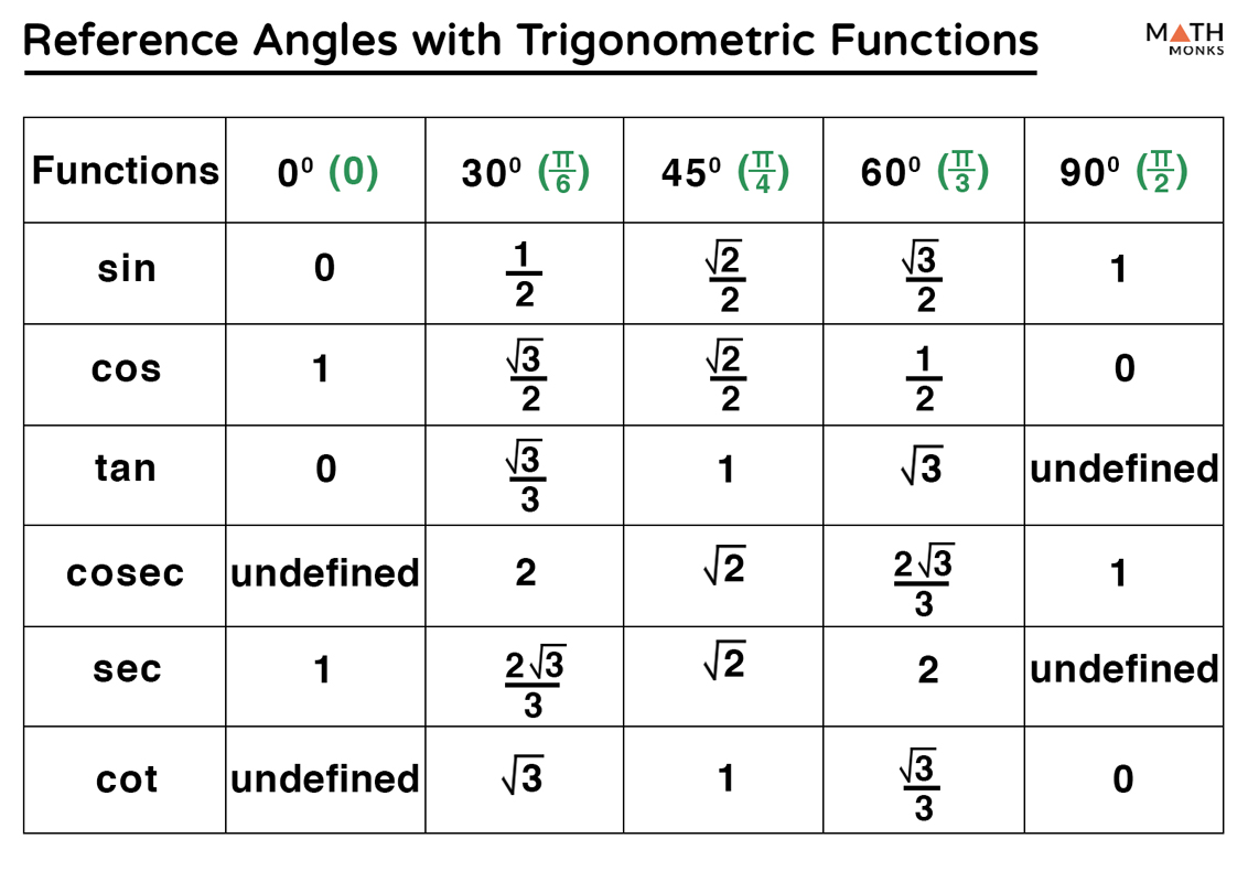
If an NPC has a maximum viewing angle of $45^\circ$ to either side of its center line, the threshold cosine value is $\cos(45^\circ) \approx 0.7071$.
- If $\mathbf{u} \cdot \mathbf{v} \ge 0.7071$, the player is within the field of view.
- If $\mathbf{u} \cdot \mathbf{v} < 0.7071$, the player is outside the field of view.
This dot-product comparison avoids calling the computationally expensive inverse cosine function ($\arccos$) thousands of times per frame.
Two-Argument Arctangent (atan2) in Autonomous Navigation
Standard inverse tangent ($\arctan(y/x)$) returns values only within the range of $-\frac{\pi}{2}$ to $+\frac{\pi}{2}$ (quadrants I and IV), losing information about the true quadrant of the vector because the ratio $(-y)/(-x)$ is algebraically identical to $(+y)/(+x)$.
To resolve this limitation, computer systems implement the two-argument function atan2(y, x). This function analyzes the signs of both $x$ and $y$ independently to return the correct full-circle heading angle in the range $(-\pi, +\pi]$ radians or $[0^\circ, 360^\circ)$.
- Quadrant I (Q I):
- Coordinates: $(+x, +y)$
- Angle Range: $0^\circ$ to $90^\circ$
- Quadrant II (Q II):
- Coordinates: $(-x, +y)$
- Angle Range: $180^\circ$ to $90^\circ$
- Quadrant III (Q III):
- Coordinates: $(-x, -y)$
- Angle Range: $-180^\circ$ to $-90^\circ$
- Quadrant IV (Q IV):
- Coordinates: $(+x, -y)$
- Angle Range: $-90^\circ$ to $0^\circ$
- Axes:
- $+X$: $\pm 180^\circ / 0^\circ$
- $+Y$: $90^\circ$
- $-Y$: $-90^\circ$
Autonomous mobile robots (AMRs) compute steering corrections relative to target coordinates $(x_{\text{target}}, y_{\text{target}})$ and robot coordinates $(x_{\text{robot}}, y_{\text{robot}})$ using atan2:
$$\Delta x = x_{\text{target}} - x_{\text{robot}}$$ $$\Delta y = y_{\text{target}} - y_{\text{robot}}$$ $$\text{Desired Heading} = \text{atan2}(\Delta y, \Delta x)$$
Angle Addition, Subtraction, and Coordinate Rotations
Angle addition and subtraction identities decompose composite rotational values into discrete wave parameters or transformation terms.
Fundamental Identities
$$\sin(\alpha \pm \beta) = \sin\alpha \cos\beta \pm \cos\alpha \sin\beta$$ $$\cos(\alpha \pm \beta) = \cos\alpha \cos\beta \mp \sin\alpha \sin\beta$$ $$\tan(\alpha \pm \beta) = \frac{\tan\alpha \pm \tan\beta}{1 \mp \tan\alpha \tan\beta}$$
Rotating Points in 2D Space
In computer-aided design (CAD) software and image processing algorithms, rotating a point $(x, y)$ around the origin by an angle $\theta$ relies directly on the angle addition formulas.
- Origin $(0, 0)$
- Point $P(x, y)$ at initial angle $\phi$ relative to the X-axis
- Point $P'(x', y')$ rotated counterclockwise from point $P$ by angle $\theta$
Let the initial point $P$ sit at a distance $r$ from the origin with an initial orientation angle $\phi$:
$$x = r \cos(\phi)$$ $$y = r \sin(\phi)$$
When rotating the point counterclockwise by an additional angle $\theta$, the new coordinates $(x', y')$ become:
$$x' = r \cos(\phi + \theta)$$ $$y' = r \sin(\phi + \theta)$$
Applying the cosine addition identity to $x'$:
$$x' = r (\cos\phi \cos\theta - \sin\phi \sin\theta) = (r \cos\phi) \cos\theta - (r \sin\phi) \sin\theta$$
Substituting $x = r \cos\phi$ and $y = r \sin\phi$:
$$x' = x \cos\theta - y \sin\theta$$
Applying the sine addition identity to $y'$:
$$y' = r (\sin\phi \cos\theta + \cos\phi \sin\theta) = (r \sin\phi) \cos\theta + (r \cos\phi) \sin\theta$$ $$y' = y \cos\theta + x \sin\theta$$
In matrix notation, this forms the standard 2D Rotation Matrix used universally across graphics libraries:
$$\begin{bmatrix} x' \ y' \end{bmatrix} = \begin{bmatrix} \cos\theta & -\sin\theta \ \sin\theta & \cos\theta \end{bmatrix} \begin{bmatrix} x \ y \end{bmatrix}$$
Common Pitfalls and Edge Cases in Applied Trigonometry
Applying trigonometric theory to real-world software or field environments introduces numerical and practical failure points. Addressing these edge cases prevents field errors and application crashes.
1. Degree vs. Radian Execution Errors
Most programming languages (C++, Python, Java, JavaScript) process standard mathematical functions (sin(), cos(), tan()) strictly in radians, whereas physical hardware displays (such as total station transits or aviation indicators) typically read in degrees.
- Conversion Formulas: $$\text{Radians} = \text{Degrees} \times \frac{\pi}{180}$$ $$\text{Degrees} = \text{Radians} \times \frac{180}{\pi}$$
Executing math.sin(45) in Python evaluates 45 radians (approx. 0.8509) rather than 45 degrees ($\sin(45^\circ) \approx 0.7071$).
2. Floating-Point Domain Errors in Inverse Cosine (acos)
The mathematical domain of $\arccos(x)$ is strictly restricted to $-1.0 \le x \le 1.0$. In computational implementations of the vector dot product or Law of Cosines:
$$\text{ratio} = \frac{\mathbf{u} \cdot \mathbf{v}}{|\mathbf{u}| |\mathbf{v}|}$$
Due to IEEE 754 floating-point rounding errors, two perfectly collinear vectors might evaluate to a ratio like 1.0000000000000002. Passing this value into acos() produces a NaN (Not a Number) domain error or throws an runtime exception.
Practical Remedy: Clamp input values explicitly before calling inverse functions:
ratio = max(-1.0, min(1.0, calculated_ratio)) angle = math.acos(ratio)
3. Gimbal Lock in 3D Euler Angles
When concatenating individual 3D rotational angles (pitch, yaw, roll) using standard trigonometric rotation matrices, aligning two axes of rotation causes the loss of one degree of freedom—a state known as gimbal lock.
- Normal 3D Movement (3 Independent Axes):
- Pitch (X)
- Yaw (Y)
- Roll (Z)
- Gimbal Lock State (Pitch Axis Aligns with Yaw):
- Pitch and Yaw axes become collinear
- Roll (Z) axis remains
- Result: 1 Degree of Freedom LOST
To bypass gimbal lock in 3D spatial software, navigation systems, and game development, systems replace sequential trigonometric Euler angles with Quaternions—four-element hypercomplex numbers that interpolate 3D rotations smoothly without trigonometric singularities.
Frequently Asked Questions
What is the difference between right-triangle trigonometry and oblique trigonometry?
Right-triangle trigonometry applies exclusively to triangles containing one $90^\circ$ angle, utilizing simple sine, cosine, and tangent ratios. Oblique trigonometry applies to triangles without a $90^\circ$ interior angle, requiring broader relationships like the Law of Sines or Law of Cosines.
When should I use the Law of Cosines instead of the Law of Sines?
Use the Law of Cosines when you know all three side lengths (SSS) and need to calculate an interior angle, or when you know two sides and the included angle between them (SAS). Use the Law of Sines when you know two angles and any side (AAS or ASA), or two sides and a non-included opposite angle (SSA).
Why do software developers use atan2(y, x) instead of atan(y/x)?
The standard atan(ratio) function returns angles strictly between $-90^\circ$ and $+90^\circ$, making it impossible to distinguish between opposite directions (e.g., Quadrant I vs. Quadrant III). The atan2(y, x) function takes $y$ and $x$ coordinates as separate arguments, evaluating their arithmetic signs to determine the exact quadrant across a full $360^\circ$ range.
How are angle formulas used in structural civil engineering?
Civil engineers use angle formulas to calculate force vector resolution in structural trusses, measure land grade percentages, design banked roadway curves to balance centripetal acceleration, and evaluate load distributions across angled support beams.
How do floating-point precision issues affect trigonometric calculations in software?
Because computers store real numbers using finite floating-point representations, calculated values intended to equal $1.0$ can evaluate slightly higher (e.g., $1.0000001$). Passing these out-of-bounds values into domain-restricted functions like acos() or asin() causes computational errors or NaN outputs. Programmers prevent this by clamping inputs to $[-1.0, 1.0]$.
Practical Implementation Steps
To incorporate trigonometric angle formulas reliably into applied workflows, adopt the following structured sequence:
- Classify the Spatial System: Determine whether your environment permits a right-triangle setup, requires oblique geometric laws, or relies on 2D/3D vector spaces.
- Normalize Input Units: Standardize all inputs before computing. If working in physical surveying, convert degrees-minutes-seconds (DMS) into decimal degrees. If writing computational scripts, convert decimal degrees into radians using $\text{Radians} = \text{Degrees} \times \frac{\pi}{180}$.
- Select the Computationally Stable Formula:
- For single right triangles: Use standard ratios ($\tan, \sin, \cos$).
- For coordinate-based headings: Use
atan2(y, x)rather thanatan(y/x). - For vector alignments: Use normalized dot products ($\mathbf{u} \cdot \mathbf{v}$).
- Implement Defensive Boundary Checks: Clamp inputs to functions like
arccos()to $[-1.0, 1.0]$, and check for zero-length vectors before calculating magnitude denominators to prevent division-by-zero errors. - Verify Quadrant Integrity: Verify that output angles fall into the expected spatial quadrant, adding $360^\circ$ ($2\pi$) if negative outputs require mapping to standard positive azimuths ($0^\circ \text{ to } 360^\circ$).