The primary difference between ARIMA and ARMA lies in how they handle data trends. ARMA (Autoregressive Moving Average) is designed strictly for stationary time series, where statistical properties like mean and variance are constant over time. ARIMA (Autoregressive Integrated Moving Average) adds an "Integrated" component, allowing it to handle non-stationary data by applying differencing to stabilize the series.
In the realm of statistical forecasting and econometrics, selecting the correct model is the difference between a high-accuracy prediction and a fundamentally flawed projection. As we operate in 2026, these classical models remain the bedrock of time series analysis, even alongside advanced neural networks, due to their interpretability and efficiency in handling structured financial and physical data.
Understanding the Fundamentals of ARMA Models
The ARMA model is a hybrid statistical tool used to describe stationary stochastic processes. To understand ARMA, one must decompose it into its two core components: the Autoregressive (AR) part and the Moving Average (MA) part.
The Autoregressive (AR) Component
The "AR" in ARMA stands for Autoregression. In an AR model, the current value of a variable is predicted based on its own previous values (lags). If we denote the current value as $Y_t$, an AR model of order $p$—written as AR(p)—assumes that $Y_t$ is a linear combination of $Y_{t-1}, Y_{t-2}, \dots, Y_{t-p}$. This is essentially a regression where the independent variables are the historical observations of the dependent variable.
This component captures the "momentum" or "memory" of a dataset. For example, if a temperature reading today is highly correlated with the temperature yesterday, an AR model is likely to capture that relationship effectively.
The Moving Average (MA) Component
The "MA" component, or Moving Average, focuses on the relationship between an observation and a residual error from a moving average model applied to lagged observations. An MA model of order $q$—written as MA(q)—suggests that the current value is influenced by current and past error terms (shocks).
Unlike a simple moving average used in technical analysis (which smooths out data), the MA component in ARMA is about error correction. It helps the model account for unpredictable "shocks" to the system—such as a sudden market shift or an unexpected weather event—and how those shocks dissipate over time.
The Requirement for Stationarity
The most critical limitation of the ARMA model is the prerequisite of stationarity. For ARMA to function, the data must exhibit a constant mean, constant variance, and an autocovariance that does not depend on time. If your data has a visible trend (upward or downward) or seasonality, a standard ARMA model will produce unreliable results because it cannot mathematically account for a shifting baseline.
The Evolution to ARIMA: Adding the "I" Factor
As researchers encountered real-world data, they realized that pure stationarity is rare. Stock prices, GDP growth, and population metrics almost always exhibit trends. This led to the development of the ARIMA model, which introduces the concept of "Integration" (the "I" in ARIMA).
What is Integration (Differencing)?
The "Integrated" part of ARIMA refers to differencing. Differencing is the process of subtracting the previous observation from the current observation ($Y_t - Y_{t-1}$). This simple mathematical transformation is incredibly powerful: it can remove trends and stabilize the mean of a time series.
If a series has a linear trend, one round of differencing (first-order differencing) usually makes it stationary. If the trend is quadratic or more complex, a second round of differencing may be required. The number of times the data must be differenced to achieve stationarity is denoted by the parameter $d$.
The Notation: p, d, and q
ARIMA models are defined by three parameters:
- p (AR): The number of lag observations included in the model.
- d (I): The number of times that the raw observations are differenced.
- q (MA): The size of the moving average window.
An ARIMA(1, 1, 1) model, for instance, includes one lag of the variable, one level of differencing, and one lag of the forecast error. If you set $d=0$ in an ARIMA model, it simplifies exactly into an ARMA model. Therefore, ARMA is essentially a special case of ARIMA.
Direct Comparison: ARIMA vs. ARMA
To choose the right model, one must evaluate the nature of the dataset. The following table summarizes the primary distinctions that analysts use to differentiate these two approaches.
| Feature | ARMA | ARIMA |
|---|---|---|
| Full Name | Autoregressive Moving Average | Autoregressive Integrated Moving Average |
| Components | AR(p) + MA(q) | AR(p) + I(d) + MA(q) |
| Data Requirement | Must be stationary from the start | Can handle non-stationary data (trends) |
| Primary Use Case | Short-term fluctuations in stable systems | Economic forecasting, stock trends, growth metrics |
| Mathematical Goal | Model noise and momentum | Remove trends then model noise and momentum |
| Complexity | Lower; fewer parameters to tune | Higher; requires determining the order of $d$ |
| Handling Trends | Fails if a trend is present | Successfully removes trends via differencing |
Identifying the Need for Differencing
The most frequent question in 2026 time series analysis remains: "How do I know if I need ARIMA or if ARMA is sufficient?" This decision rests entirely on the Unit Root Test.
Visual Diagnostics
Before running formal tests, analysts often look at a time plot of the data. If the data drifts upward or downward over time, or if the variance increases as time progresses, it is non-stationary. Additionally, the Autocorrelation Function (ACF) plot for non-stationary data typically shows a very slow decay, indicating that the observations are heavily dependent on their distant past due to an underlying trend.
Statistical Tests (ADF and KPSS)
To move beyond visual guesswork, two primary tests are used:
- Augmented Dickey-Fuller (ADF) Test: This test checks for a unit root. The null hypothesis is that the series is non-stationary. A low p-value (typically < 0.05) suggests the data is stationary and ARMA may be used.
- KPSS Test: This is the inverse of the ADF test. The null hypothesis is that the series is stationary. If the p-value is low, you must difference the data, necessitating an ARIMA approach.
In professional practice, it is common to use both. If both tests agree the data is non-stationary, the "I" component of ARIMA is mandatory.
Practical Implementation Steps
Regardless of whether you choose ARMA or ARIMA, the modeling process follows the Box-Jenkins Methodology, which consists of four iterative steps.
1. Model Identification
This involves determining the values of $p, d,$ and $q$. Using tools like the ACF and Partial Autocorrelation Function (PACF) plots, you can estimate the initial orders. For example, if the PACF cuts off after lag $p$ and the ACF decays exponentially, an AR(p) model is suggested. In 2026, many analysts utilize automated algorithms like auto.arima in R or pmdarima in Python, which iterate through various combinations of $p, d,$ and $q$ to find the optimal fit based on information criteria.
2. Parameter Estimation
Once the orders are identified, the model coefficients are estimated. This is usually done through Maximum Likelihood Estimation (MLE), which finds the parameter values that maximize the probability of observing the given data.
3. Diagnostic Checking (Residual Analysis)
After fitting the model, you must examine the residuals (the errors). If the model is a good fit, the residuals should behave like white noise. This means:
- The residuals should have no autocorrelation (checked via the Ljung-Box test).
- The residuals should have a mean of zero.
- The residuals should have constant variance.
If the residuals show patterns, it indicates that the model has failed to capture some information, and you may need to adjust the $p, q$, or $d$ parameters.
4. Forecasting
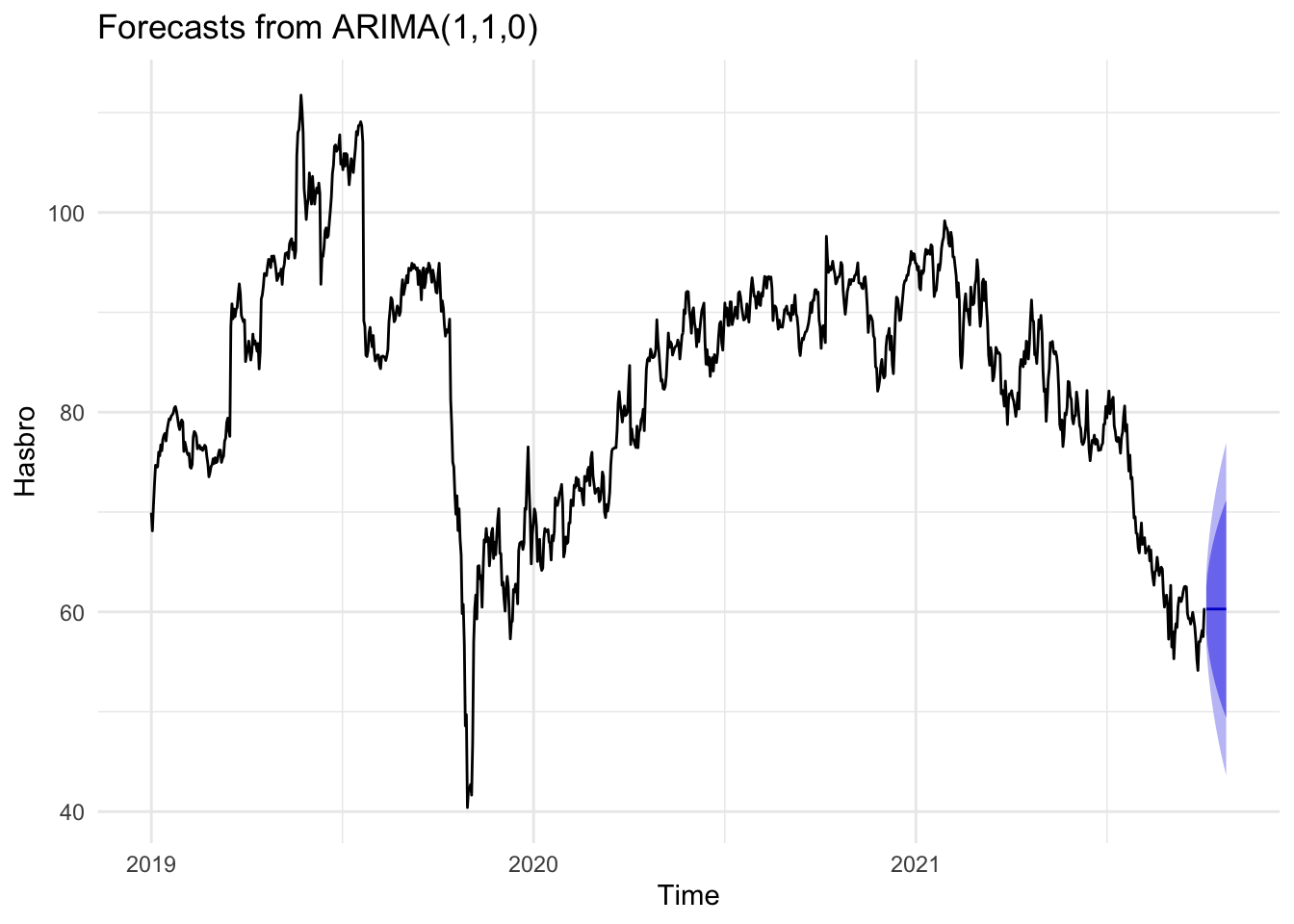
Once validated, the model can project future values. It is important to note that ARIMA/ARMA models are generally better for short-to-medium term forecasting. In long-term horizons, the confidence intervals tend to widen significantly, reflecting the inherent uncertainty in stochastic processes.
Advanced Variations: Beyond Standard ARIMA
In many real-world scenarios, a basic ARIMA model is still insufficient. Several extensions have been developed to handle specific data complexities.
SARIMA (Seasonal ARIMA)
Standard ARIMA cannot handle seasonality (e.g., retail sales spiking every December). SARIMA adds seasonal AR, I, and MA terms. It is denoted as ARIMA(p, d, q)(P, D, Q)m, where $m$ is the number of periods in each season (e.g., 12 for monthly data).
ARIMAX (ARIMA with Exogenous Variables)
Sometimes, an external factor influences the time series. For example, local temperature might influence electricity demand. ARIMAX allows for the inclusion of external regressors, combining the time-series capabilities of ARIMA with the explanatory power of linear regression.
ARCH and GARCH
While ARIMA focuses on the mean of the series, ARCH (Autoregressive Conditional Heteroskedasticity) and GARCH models focus on the variance (volatility). These are often used in finance in conjunction with ARIMA to model "volatility clustering," where periods of high volatility are followed by further high volatility.
Common Pitfalls and Troubleshooting
Even with sophisticated software, errors in model selection are common.
- Over-differencing: Applying differencing ($d > 1$) when it isn't necessary can introduce artificial patterns into the data and lead to poor forecasts. Always test for stationarity before differencing.
- Overfitting: Including too many lags ($p$ or $q$) can make the model fit the "noise" of the historical data perfectly but fail miserably when predicting new, unseen data. Always prefer the simplest model that passes diagnostic tests (the principle of parsimony).
- Ignoring Structural Breaks: ARIMA assumes the underlying process doesn't change. However, events like a pandemic, a major policy change, or a technological breakthrough in 2026 can cause a "structural break." In such cases, the model may need to be reset or adjusted with dummy variables.
Selecting the Right Model for Your Project
The choice between ARIMA and ARMA is ultimately a choice about the stability of your data. If your data represents a system in equilibrium—such as the white noise of a signal or the steady-state fluctuations of a controlled industrial process—ARMA is the more efficient, elegant choice.
However, if you are dealing with "living" data—economic indicators, social trends, or market prices—ARIMA is almost always necessary to account for the inevitable drifts and shifts inherent in human and natural systems. By identifying the order of integration first, you ensure that your model is built on a stable, stationary foundation, allowing the AR and MA components to accurately capture the remaining dynamics.
For most modern applications, starting with a test for stationarity is the standard protocol. If the test fails, proceed with ARIMA; if it passes, ARMA will suffice.
Frequently Asked Questions
Can I use ARMA for stock price prediction? Generally, no. Stock prices are typically non-stationary (they follow a random walk or have trends). You would need to use at least a first-order ARIMA model (specifically, differencing the prices to get returns) or more advanced models like GARCH to handle the volatility.
What is the difference between ARIMA and SARIMA? ARIMA is designed for non-seasonal data. SARIMA (Seasonal ARIMA) extends ARIMA by adding seasonal components to account for patterns that repeat at regular intervals, such as daily, weekly, or monthly cycles.
How do I choose the optimal p, d, and q values? The most common method is to minimize the Akaike Information Criterion (AIC) or the Bayesian Information Criterion (BIC). These metrics reward models that fit the data well but penalize models with too many parameters, helping to prevent overfitting.
Is ARIMA still relevant in 2026 with the rise of AI? Yes. While Deep Learning models like LSTMs (Long Short-Term Memory) and Transformers are powerful, ARIMA remains highly relevant because it requires significantly less data, is computationally "cheaper," and provides a clear mathematical explanation for its predictions, which is critical in regulated industries like finance and healthcare.
What does it mean if my d value is 0? If $d=0$, the model is not performing any differencing. This means your data is already stationary, and your ARIMA(p, 0, q) model is functionally identical to an ARMA(p, q) model.