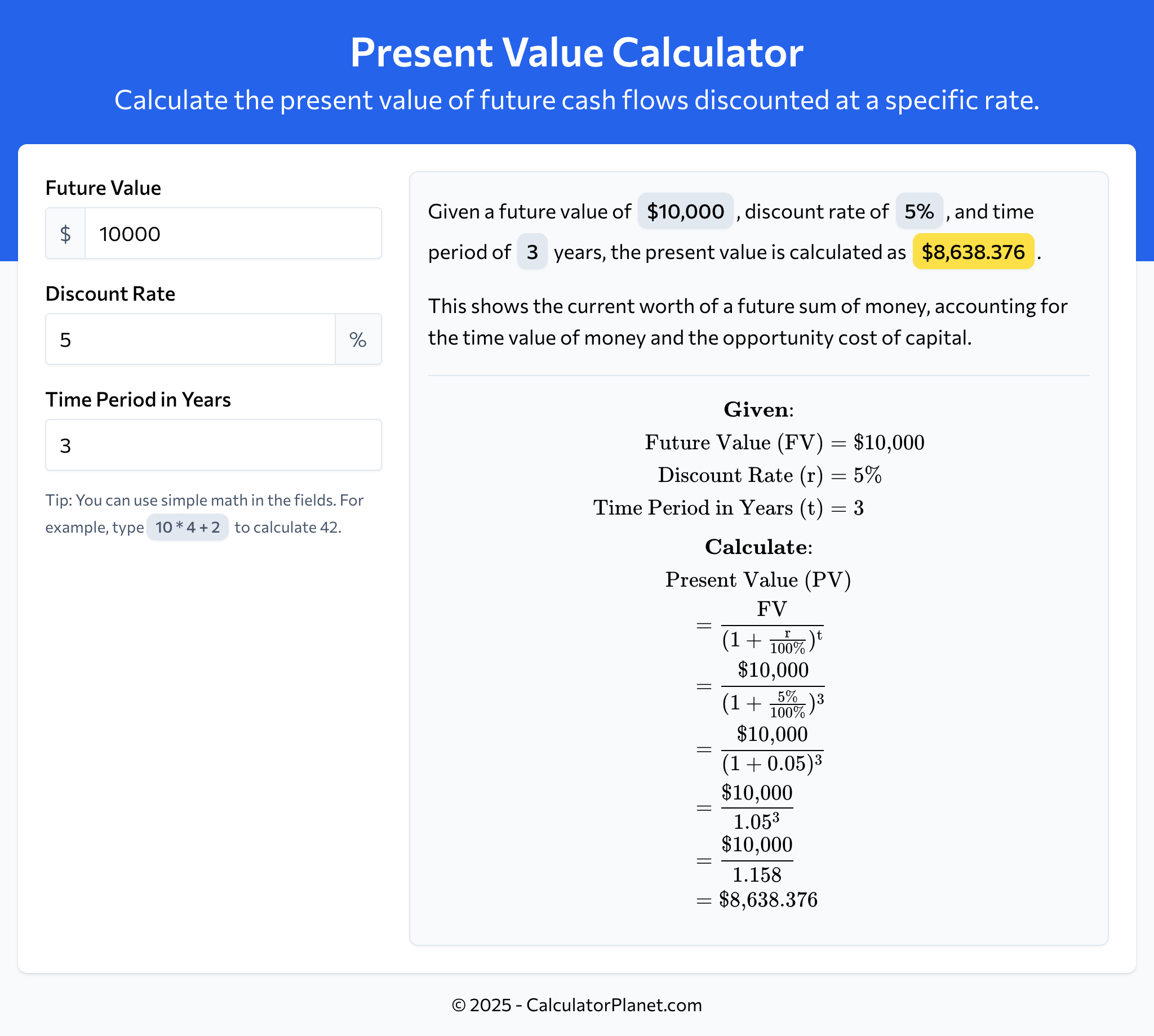
A 10-year net present value calculation determines the current value of a stream of cash flows projected over a decade by discounting them back to today's dollars using a specific rate of return, helping investors and businesses evaluate long-term profitability.
Evaluating long-term financial projects, capital investments, real estate developments, or business expansions requires tools that account for the changing value of money over time. A standard financial method used by analysts, CFOs, and individual investors is the Net Present Value (NPV) calculation. When projected over a ten-year horizon, this calculation acts as a financial stress test, weighing immediate capital outlays against a decade of future operational cash flows. Because a dollar today is worth more than a dollar ten years from now due to inflation and opportunity cost, discounting future cash flows is vital for making sound capital allocation decisions.
Understanding how to build, execute, and interpret a 10-year net present value calculation requires mastering its underlying mathematical framework, recognizing the core variables involved, and knowing how to interpret the final output. Financial analysis demands precision, transparency regarding assumptions, and an appreciation of the limitations inherent in long-term forecasting.
The Core Concept of Net Present Value (NPV)
At its foundation, NPV measures the total value created or destroyed by an investment over a designated period. It translates future cash inflows and outflows into a single, consolidated present-day figure. If the resulting NPV is positive, the investment is expected to generate more value than its initial cost, exceeding the required rate of return. If the NPV is negative, the project will destroy value relative to that benchmark.
The foundational principle driving NPV is the time value of money. Capital can be deployed elsewhere to earn a return, such as in government bonds, public equities, or alternative business ventures. Therefore, future money must be discounted to reflect this lost opportunity. Over a 10-year timeline, this discounting effect becomes pronounced. Cash flows arriving in year nine or ten are heavily discounted compared to cash flows arriving in year one or two, making long-term forecasting particularly sensitive to the chosen discount rate.
The Mathematical Formula
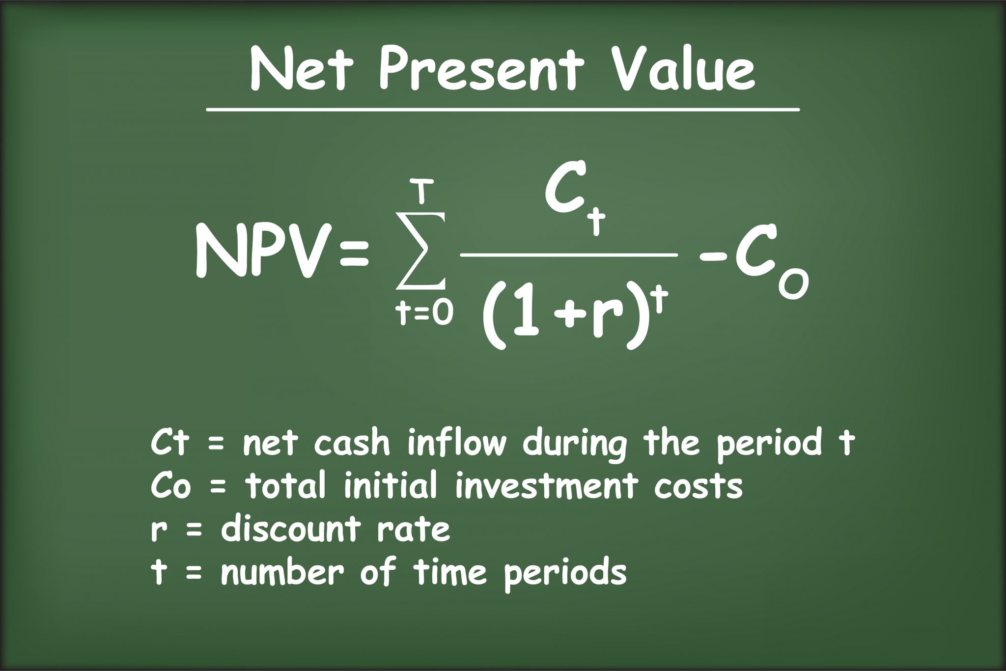
The mathematical expression for a 10-year net present value calculation is an expansion of the standard discounted cash flow equation:
$$NPV = \sum_{t=1}^{10} \frac{CF_t}{(1 + r)^t} - C_0$$
Where:
- $CF_t$ = Net cash flow during a single period $t$ (from year 1 through year 10)
- $r$ = Discount rate or hurdle rate
- $t$ = Number of time periods (years 1 to 10)
- $C_0$ = Total initial investment or initial cash outflow at time zero
To perform this manually, each annual cash flow is divided by one plus the discount rate raised to the power of the corresponding year number. The sum of these ten discounted values is then reduced by the initial capital expenditure.
Prerequisites and Key Variables for a 10-Year Model
Building an accurate 10-year financial model requires gathering precise inputs. Errors or overly optimistic assumptions in the early stages of data collection will cascade through a decade of calculations, distorting the final output.
1. Initial Outlay ($C_0$)
This represents all cash spent at the inception of the project to get it running. It includes asset purchases, equipment acquisition, legal fees, site preparation, and initial working capital requirements. This figure is entered as a negative number in the formula because it represents cash leaving the business.
2. Annual Cash Flows ($CF_t$)
For each of the ten years, the model requires an estimate of the net cash generated or consumed. Net cash flow is distinct from net income; it starts with operating income, adds back non-cash expenses like depreciation and amortization, adjusts for changes in working capital, and subtracts capital expenditures required to maintain operations throughout the decade.
3. The Discount Rate ($r$)
Selecting the discount rate is the most critical and often most subjective step in the process. The discount rate reflects the risk profile of the project and the opportunity cost of capital. Corporations typically use their Weighted Average Cost of Capital (WACC) as a baseline, adjusting it upward for riskier ventures or downward for highly stable, regulated projects. Individual investors might use their target rate of return or the yield available on comparable alternative investments.
Step-by-Step Execution of a 10-Year Calculation
Executing the model follows a structured progression from data gathering to final interpretation. While financial software or spreadsheet applications automate the arithmetic, understanding the mechanical steps ensures the integrity of the model.
- Gather Initial Outlay & WACC
- Forecast 10 Years of Net Cash Flows
- Apply Discount Factor to Each Year: $CF / (1 + r)^t$
- Sum All Discounted Cash Flows
- Subtract Initial Outlay to Arrive at Final NPV
Step 1: Establish the Baseline Assumptions
Document all underlying macroeconomic and operational assumptions. Define the projected revenue growth rates, cost of goods sold (COGS) inflation, operating expense scaling, tax rates, and salvage values at the end of year ten.
Step 2: Project Year-by-Year Cash Flows
Draft a schedule from Year 1 through Year 10. List revenues, subtract operating expenses, account for taxes, adjust for non-cash items, and factor in ongoing capital expenditures (CapEx) for maintenance or replacement of equipment. The resulting line is the net cash flow for that specific year.
Step 3: Calculate the Discount Factor for Each Year
For each of the ten years, compute the discount factor using the chosen rate ($r$). For example, if the discount rate is 8% ($0.08$):
- Year 1 Discount Factor: $\frac{1}{(1 + 0.08)^1} = 0.9259$
- Year 2 Discount Factor: $\frac{1}{(1 + 0.08)^2} = 0.8573$
- Year 10 Discount Factor: $\frac{1}{(1 + 0.08)^{10}} = 0.4632$
Step 4: Discount the Cash Flows
Multiply each year’s projected net cash flow by its corresponding discount factor. This converts nominal future dollars into real present-day equivalents.
Step 5: Aggregate and Subtract Initial Investment
Sum the ten discounted cash flows together. Finally, subtract the initial capital outlay ($C_0$) incurred at Year 0. The resulting number is the 10-year net present value.
Illustrative 10-Year NPV Scenario
To observe how this functions in practice, consider a commercial real estate or equipment investment requiring an initial outlay of $1,000,000. The investor mandates a 10% discount rate. The project generates varying cash flows over a decade as operations scale, plateau, and eventually require facility overhauls.
| Year | Projected Cash Flow | Discount Factor (10%) | Present Value of Cash Flow |
|---|---|---|---|
| Year 0 | ($1,000,000) | 1.0000 | ($1,000,000) |
| Year 1 | $120,000 | 0.9091 | $109,092 |
| Year 2 | $150,000 | 0.8264 | $123,960 |
| Year 3 | $180,000 | 0.7513 | $135,234 |
| Year 4 | $200,000 | 0.6830 | $136,600 |
| Year 5 | $220,000 | 0.6209 | $136,598 |
| Year 6 | $250,000 | 0.5645 | $141,125 |
| Year 7 | $250,000 | 0.5132 | $128,300 |
| Year 8 | $240,000 | 0.4665 | $111,960 |
| Year 9 | $220,000 | 0.4241 | $93,302 |
| Year 10 | $200,000 | 0.3855 | $77,100 |
| Total | $1,050,000 | — | $193,271 |
In this scenario, while the nominal sum of cash flows over ten years is $1,050,000 against an initial cost of $1,000,000 (suggesting a raw profit of $50,000), the time value of money changes the perspective. When discounted at 10% per year, the present value of the inflows equals $1,193,271. Subtracting the initial $1,000,000 yields a positive NPV of $193,271. This confirms that the project exceeds the 10% hurdle rate and creates economic value.
Advantages and Limitations of a 10-Year Horizon
While a 10-year net present value calculation provides deep insight into long-term ventures, analysts must weigh its strengths against its structural limitations.
Advantages
- Accounts for the Time Value of Money: Unlike simple payback periods or return on investment (ROI) metrics that ignore timing, NPV explicitly weighs when cash enters and leaves the business.
- Comprehensive Long-Term View: A 10-year window captures full business cycles, maturation phases of projects, and structural shifts that short-term 3-to-5-year models miss.
- Absolute Value Creation: NPV provides an absolute monetary figure ($) representing wealth creation, allowing decision-makers to compare projects of varying scales.
Limitations
- Forecasting Uncertainty: Projecting cash flows accurately across a decade is inherently difficult. Technological disruptions, regulatory changes, and macroeconomic shifts can render year-nine and year-ten estimates inaccurate.
- Sensitivity to Discount Rate: A minor adjustment in the discount rate can flip a project from profitable to unviable, particularly in later years where discounting compounds heavily.
- Static Assumptions: Traditional NPV models assume fixed discount rates and constant risk profiles over ten years, whereas real-world risk profiles evolve dynamically.
Best Practices and Sensitivity Analysis
Because forecasting a decade into the future introduces substantial estimation risk, experienced analysts never rely on a single NPV output. Instead, they use complementary analytical techniques to stress-test the model.
Conducting Sensitivity Analysis
Sensitivity analysis involves altering key variables—such as revenue growth rates, operating margins, or the discount rate—to observe their impact on the final NPV. For instance, testing the model with a discount rate 200 basis points higher than baseline reveals whether the project remains viable if borrowing costs rise.
Scenario Modeling
Construct three distinct versions of the 10-year model:
- Base Case: Most realistic operational trajectory based on current data.
- Optimistic Case: Higher revenue growth and lower operational costs.
- Conservative/Downside Case: Slower adoption, margin compression, or inflationary cost pressures.
Evaluating the NPV across these scenarios establishes a risk corridor, ensuring capital is not deployed based on an outlier best-case projection.
Frequently Asked Questions
What is the difference between NPV and IRR?
Net Present Value calculates the absolute monetary value added by an investment in today's dollars, assuming a specific discount rate. Internal Rate of Return (IRR) calculates the annualized effective compound return rate that forces the NPV of all cash flows to zero. While IRR provides a percentage yield, NPV measures actual wealth generation, making NPV superior for choosing between mutually exclusive projects of different sizes.
How do I handle terminal value in a 10-year model?
If a project or business is expected to continue generating cash flows beyond the 10-year mark, analysts often calculate a Terminal Value (TV) at the end of Year 10. This is typically done using the Gordon Growth Model (perpetuity growth method) or an exit multiple method. The resulting terminal value is then discounted back from Year 10 to present day using the discount factor and added to the cumulative NPV of the first ten years.
What discount rate should I use for a 10-year projection?
Corporations typically use their Weighted Average Cost of Capital (WACC), which blends the cost of debt and equity financing. For independent real estate or entrepreneurial projects, the discount rate should reflect the investor's required rate of return, factoring in risk premiums for the specific industry, illiquidity, and market volatility.
Can inflation be built directly into cash flow projections?
Yes. Analysts can either use nominal cash flows combined with a nominal discount rate that includes inflation, or real cash flows combined with a real discount rate that strips out inflation. Consistency is critical: mixing nominal cash flows with a real discount rate will invalidate the calculation.
Conclusion and Next Actions
Executing a robust 10-year net present value calculation requires a disciplined approach to gathering initial outlay data, projecting multi-year operational cash flows, and selecting an appropriate discount rate. To apply these principles effectively, begin by building a flexible spreadsheet model where cash flows and discount rates can be adjusted dynamically. Run multiple scenarios to account for long-term forecasting uncertainty, and always evaluate the resulting NPV alongside qualitative strategic factors before committing capital to any decade-long initiative.